Cloud masking with native OmniCloudMask
omnicloudmask.RmdOmniCloudMask is a state-of-the-art cloud and cloud-shadow segmentation model: two convolutional U-Nets that read only red, green, and NIR and return, per pixel, one of four classes (0 clear, 1 thick cloud, 2 thin cloud, 3 shadow). It routinely beats the quality masks that ship with the imagery, and for serious compositing that difference is decisive.
garry runs OmniCloudMask natively. The published model weights are read directly from their safetensors files and the full two-model ensemble is expressed in garry’s own kernel vocabulary, so it compiles through anvl/XLA like every other pipeline stage: no Python, no torch, no extra runtime. The port is verified against the reference implementation to float precision (logits agree to ~1e-6), and the compiled kernel is about twice as fast as torch on CPU, more on a GPU.
The weights belong to the OmniCloudMask authors and are not shipped
with garry: download them once with ocm_fetch_weights()
(about 58 MB, hash-verified) and ocm_model() finds them
automatically. It can also read the Python package’s download cache or
any directory you point it at (see ?ocm_load_weights).
This vignette reproduces the classic OmniCloudMask demonstration (after the OCM article in the vrtility package) on garry: Zurich in spring, with scenes up to 80% cloud deliberately included, comparing OmniCloudMask against Sentinel-2’s scene classification (SCL) all the way to the composite.
A deliberately awful stack of scenes
library(garry)

bbox <- c(8.41, 47.32, 8.61, 47.44)     # Zurich, ~15 x 13 km
mpc <- "https://planetarycomputer.microsoft.com/api/stac/v1/"

items <- stac_query(bbox = bbox, stac_source = mpc,
                    collection = "sentinel-2-l2a",
                    start_date = "2024-04-01", end_date = "2024-05-30") |>
  stac_sign_mpc() |>
  stac_filter_cloud(80) |>              # keep genuinely cloudy scenes
  stac_drop_duplicates()
length(items$features)
#> [1] 9

remote <- lazy_dataset(
  items, grid = grid_from_bbox(bbox, res = 10),
  assets = c("B02", "B03", "B04", "B08", "SCL"),
  mask_asset = "SCL",
  nodata = c(B02 = 0, B03 = 0, B04 = 0, B08 = 0, SCL = 0),
  resampling = "bilinear"                # the mask band always reads near
)
Download once, mask twice
Everything below reads every band of every scene more than once: two
masking routes, per-date looks, and two composites. Rather than pull the
pixels from the Planetary Computer each time, checkpoint the warped
stack locally: materialise() executes the graph into
garry’s raw-BSQ cube format (one multiband .vrt +
.bin per date, readable by any GDAL tool and re-read by
garry much faster than tiled GeoTIFF) through ONE plan, and returns the
same lazy dataset rebuilt over the local files with band names, slice
dates, and the mask_asset intact. By default the cubes land
in a unique session-temporary directory, announced as it runs; give
dir a real path to keep or reuse them. From here on,
nothing touches the network.
ds <- materialise(remote)
#> materialising to '/tmp/RtmpgupY8G/materialise-1129e222133090'
#> (session-temporary)
ds
#> ── <LazyDataset> ───────────────────────────────────────────────────────────────
#>   bands  B02 B03 B04 B08  (+SCL)
#>   time   9 slices
#>   grid   1514 x 1336 • f32
#>   crs    Lambert Azimuthal Equal Area
#>   graph  45 nodes • lazy
#>   ℹ draw(x) to see the pipeline
What the two masks see
Load the model once; it is reusable across any number of scenes and datasets, and every per-slice masking stage below shares one compiled kernel.
m <- ocm_model()
m
#> $fn
#> function (x)
#> .ocm_infer(x, weights)
#> <bytecode: 0x5824aca43350>
#> <environment: 0x5824aca46cb0>
#>
#> $kernel_id
#> [1] "ocm-6709c94dbdec4de35b51a4a36ccd4e6a-regnety+edgenext"
#>
#> $halo
#> [1] 128
#>
#> $bytes_px
#> [1] 700
#>
#> $flops_px
#> [1] 80000
#>
#> $models
#> [1] "regnety"  "edgenext"
#>
#> attr(,"class")
#> [1] "garry_ocm_model"
Pick one properly cloudy date and put the scene, its SCL band, and
the OmniCloudMask classes side by side. ocm_predict() is
lazy like every garry verb: the class raster below is a graph node until
something collects it.
dates <- ds[["B04"]]@grid@labels$t       # slice dates rode through
i <- match("2024-05-25", dates)          # cumulus towers + hard shadows

slice <- function(band) time_sel(ds[[band]], i)
cls <- ocm_predict(slice("B04"), slice("B03"), slice("B08"), model = m)

rgb_i <- collect(lazy_stack(list(slice("B04"), slice("B03"), slice("B02")),
                            along = "band"))
scl_i <- collect(slice("SCL"))
ocm_i <- collect(cls)

par(mfrow = c(1, 3))
preview(rgb_i, main = "RGB", axes = FALSE)
preview(scl_i, col = hcl.colors(12, "Spectral"), main = "SCL", axes = FALSE)
preview(ocm_i, col = c("grey85", "white", "lightblue", "grey25"),
        main = "OmniCloudMask", axes = FALSE)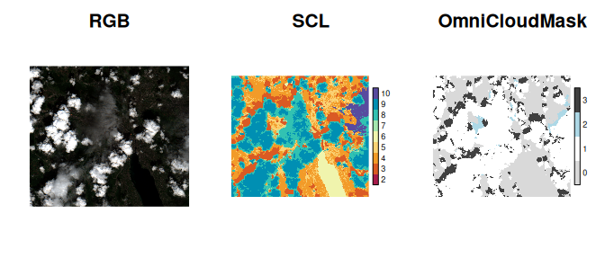
The RGB shows cumulus towers throwing hard shadows across a darkened scene. OmniCloudMask’s map reads like an annotation of it: every cloud (white) paired with its shadow (dark grey), thin fringes (blue) around the towers, clear corridors (light grey) between. The SCL band over the same pixels is a fragmented patchwork that classifies parts of the clouds as vegetation and water.
Masking a date, both ways
Route one: the local dataset carries SCL as its
mask_asset, so the standard masking call is one line (the
value set is everything SCL considers not-usable: nodata, defective,
shadows, clouds, cirrus, snow).
Route two: ocm_mask() derives the OmniCloudMask class
band from three of the dataset’s own bands, per time slice, and masks
with it through exactly the same machinery. We drop SCL first (the model
replaces it).
ocm_masked <- ds[c("B02", "B03", "B04", "B08")] |>
  ocm_mask(red = "B04", green = "B03", nir = "B08", model = m)
Same date, both masks applied, masked pixels in orange
(preview()’s na_col makes the mask footprint
explicit):
rgb_of <- function(md) collect(lazy_stack(
  list(time_sel(md[["B04"]], i), time_sel(md[["B03"]], i),
       time_sel(md[["B02"]], i)), along = "band"))
par(mfrow = c(1, 2))
preview(rgb_of(scl_masked), main = "SCL masked", axes = FALSE,
        na_col = "#eb4310")
preview(rgb_of(ocm_masked), main = "OmniCloudMask masked", axes = FALSE,
        na_col = "#eb4310")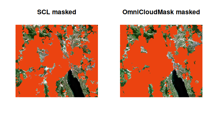
Look closely at what each mask kept. The SCL result retains more area, but bright cloud fragments are embedded in it, and patches of perfectly clear city have been thrown away; OmniCloudMask keeps the genuinely clear corridors and removes cloud and shadow together. Over a stack this costs SCL twice: fewer clean observations per pixel AND contaminated ones sneaking into what remains.
The composite is where it counts
Median-composite the two masked stacks. Residual cloud pulls a median towards bright; residual shadow pulls it dark; a good mask is the difference between a milky composite and a clean one. (Both routes are one graph each over the local cubes: reads, per-scene CNN inference, masking, and the median fuse and execute together.)
comp_of <- function(md) collect(
  reduce_over(md[c("B04", "B03", "B02")], "median", over = "t",
              nan_rm = TRUE))
scl_comp <- comp_of(scl_masked)
ocm_comp <- comp_of(ocm_masked)

par(mfrow = c(1, 2))
preview(scl_comp, main = "median of SCL-masked", axes = FALSE,
        na_col = "#eb4310")
preview(ocm_comp, main = "median of OCM-masked", axes = FALSE,
        na_col = "#eb4310")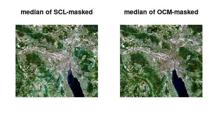
With scenes up to 80% cloud in the stack, the SCL-masked median is milky with cloud residue; the OmniCloudMask median is clean. The same comparison drives real pipelines: better masking buys more usable observations per pixel, which matters everywhere upstream of a composite, a time series, or a classification.
Two closing notes. First, everything here ran as ordinary garry graph
stages over locally materialised cubes: the CNN is subject to the same
planning, chunking, halo, and distribution as any focal or reduction,
and on a time series the per-scene inferences pipeline across the daemon
pool. Second, for composites the natural next step is the multivariate
route: reduce_over(cube, geomedian(), over = "t") on the
OCM-masked stack gives spectra no per-band median can (see the composite
vignette).