From STAC to an analysis-ready composite • garry

This is the flagship workflow: discover imagery in a STAC catalogue, describe it as a lazy dataset on an analysis grid, mask it, composite it, and stream the result to a GeoTIFF, with nothing computed until the end. The scene is the salt-working landscape around Castro Marim on the Guadiana, southern Portugal: working salinas whose crystallizer ponds read bright white against dark evaporation ponds, a tidal river, marsh, and two towns. It is photogenic, and it is also a genuinely hard compositing target: bright unstable ponds, moving water, and boats are exactly the pixels where naive composites produce spectra that never existed, which is where this vignette ends up.

Discover

stac_query() asks a STAC API for everything intersecting a bbox and date range; the filters compose directly on the returned items object. Microsoft Planetary Computer requires signed asset URLs: stac_sign_mpc() signs them, caching the collection’s token in memory and on disk until it expires, so signing is one line, once.

library(garry)

aoi <- c(-7.48, 37.19, -7.38, 37.25)   # lon/lat bbox, ~9 x 7 km
mpc <- "https://planetarycomputer.microsoft.com/api/stac/v1/"

items <- stac_query(bbox = aoi, stac_source = mpc,
                    collection = "sentinel-2-l2a",
                    start_date = "2024-01-01", end_date = "2024-12-31") |>
  stac_sign_mpc() |>
  stac_filter_cloud(30) |>            # scene-level cloud cover < 30%
  stac_drop_duplicates()
length(items$features)
#> [1] 65

Frame

Analysis happens on a grid you choose, not whichever UTM zone the data arrived in. grid_from_bbox() builds an equal-area grid over the AOI at a stated resolution; every read below warps onto it, so mixed projections, tile boundaries, and resolutions disappear at the data boundary.

target <- grid_from_bbox(aoi, res = 10)
target@dims
#>   x   y 
#> 888 667

Describe

lazy_dataset() turns items plus a band selection into a table of lazy per-date bands. Nothing is read: each entry is a promise to warp that asset onto target when execution demands it. mask_asset names the QA band; it is always read with nearest resampling regardless of the band resampling, because interpolating class codes would corrupt them.

ds <- lazy_dataset(
  items, grid = target,
  assets = c("B02", "B03", "B04", "B08"),   # blue, green, red, NIR
  mask_asset = "SCL",
  nodata = c(B02 = 0, B03 = 0, B04 = 0, B08 = 0, SCL = 0),
  resampling = "bilinear"
)
ds
#> ── <LazyDataset> ───────────────────────────────────────────────────────────────
#>   bands  B02 B03 B04 B08  (+SCL)
#>   time   65 slices
#>   grid   888 x 667 • f32
#>   crs    Lambert Azimuthal Equal Area
#>   graph  325 nodes • lazy
#>   ℹ draw(x) to see the pipeline

Mask

Sentinel-2’s scene classification (SCL) is categorical, so the mask is a value set: shadow (3), cloud medium and high probability (8, 9), cirrus (10). Raw QA rasters are speckled, and cloud edges leak: open = 2 removes mask speckle smaller than 2 px (morphological opening), and dilate = 3 grows the mask 3 px outward so translucent cloud edges go with the cloud. Masked pixels become NaN, garry’s nodata, on every value band, and the QA band is consumed.

ds <- mask(ds, where = c(3, 8, 9, 10), open = 2, dilate = 3)
ds <- (ds * 0.0001) - 0.1     # STAC raster metadata: scale, then offset
ds
#> ── <LazyDataset> ───────────────────────────────────────────────────────────────
#>   bands  B02 B03 B04 B08
#>   time   65 slices
#>   grid   888 x 667 • f32
#>   crs    Lambert Azimuthal Equal Area
#>   graph  1365 nodes • lazy
#>   ℹ draw(x) to see the pipeline

The second line is the harmonisation step readers of the asset metadata will recognise: since processing baseline 04.00 (January 2022), L2A digital numbers carry a +1000 offset ahead of the usual 1/10000 scale (raster:bands: scale 0.0001, offset -0.1). Undo both once, at the source, and everything downstream (composites, spectral distances, the written file) is in physical surface reflectance. (For collections whose files carry the affine in their band metadata, HLS for instance, lazy_dataset(scale = TRUE) discovers and applies it automatically; these Planetary Computer S2 files carry none, so the arithmetic stays explicit.)

Everything so far is graph building. draw() shows the pipeline behind any one band:

draw(ds[["B04"]])
#> ── <LazyRaster> 888 x 667 • f32 ────────────────────────────────────────────────
#> ⬚ stack  along t
#> └─ ƒ map  ×65
#>    └─ ƒ map
#>       └─ ƒ map  (2 inputs)
#>          ├─ ◈ source  888×667 f32
#>          └─ ◫ focal  r=3
#>             └─ ◫ focal  r=2
#>                └─ ◫ focal  r=2
#>                   └─ ƒ map
#>                      └─ ◈ source  888×667 f32

Composite, route one: per-band median

Reduce every band’s year to its median. Still lazy: this names a computation.

med <- reduce_over(ds, "median", over = "t", nan_rm = TRUE)

The catch hides in what “median” will do: each band reduces independently. A water pixel’s red median might come from July, its green median from March, its NIR median from November. The composite spectrum at such a pixel is a chimera that no satellite ever measured, and downstream physics (indices, unmixing, classification) inherits it. Over stable land this is harmless; over the ponds, the river, and the crystallizers, whose brightness changes week to week, it is not.

Composite, route two: the geometric median

The multivariate fix is the geometric median: per pixel, the band-vector minimising the summed spectral distance to every clean observation. It couples the bands (every distance is computed across all of them at once), so it needs to see the full band vector jointly. Stack the per-band time stacks along "band" into a (band, t, y, x) cube, and reduce that over "t" with the geomedian() reducer; the band axis survives:

cube <- lazy_stack(
  list(B02 = ds[["B02"]], B03 = ds[["B03"]],
       B04 = ds[["B04"]], B08 = ds[["B08"]]),
  along = "band")
gmed <- reduce_over(cube, geomedian(), over = "t")

Where do the two routes disagree? That question is also just more graph: subtract the composites band-wise, sum the squares over the band axis, and root it: a per-pixel spectral distance, in reflectance units.

dist <- sqrt(reduce_over((gmed - stack_bands(med))^2, "sum",
                         over = "band"))

One plan, three products

Nothing has computed yet, and nothing has been read. Start the daemon pools (a read fleet and a compute fleet, sized to the machine) and collect all three in ONE multi-export plan. Both composites consume the same source stages, so every remote asset is fetched exactly once for all three products; each composite computes once, and the distance consumes them in-plan rather than recomputing them.

garry_daemons()
res <- collect(list(median = stack_bands(med), geomedian = gmed,
                    distance = dist))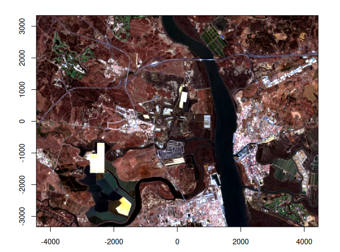

preview(res$median, bands = c(3, 2, 1))

plot of chunk sc-median

A year of tides, boats, and salt harvests collapses into one clean image.

preview(res$geomedian, bands = c(3, 2, 1))

plot of chunk sc-geomedian

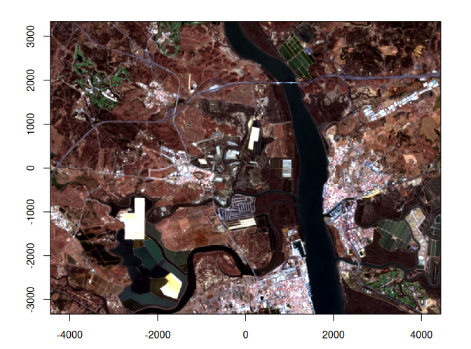
Same scene, but now every pixel’s spectrum is a genuine multivariate central tendency (solved by a fixed-iteration Weiszfeld scheme, compiled into the same chunked kernel machinery as everything else). And the distance map shows where that mattered:

preview(res$distance, stretch = c(2, 98),
        main = "median vs geomedian spectral distance")

plot of chunk sc-diff

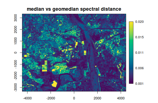
Stable land is dark (the two composites agree); the ponds, the river channel, the marsh creeks, and the crystallizers light up. Those are the pixels where the per-band median invented spectra.

If downstream analysis must only ever see observed spectra, swap in medoid(): the same construction, but the result at each pixel is the real observation nearest the geometric median, one date’s actual spectrum.

Write it out

write_tif() streams the composite to a GeoTIFF chunk by chunk as results arrive, so the full raster never needs to sit in memory; band descriptions carry through. And it can undo the reflectance scaling from the top of the pipeline: dtype = "i16" with the S2 affine quantizes each value back to a digital number at the sink, writes the scale/offset into the band metadata, and NaN becomes the sentinel. Half the bytes of float32 before compression (quantized integers also compress far better), and QGIS, GDAL, or a scale = TRUE read recover reflectance automatically. (This is a fresh plan, so it reads the scenes again; a workflow that keeps running plans over the same stack would checkpoint first with materialise(), as the OmniCloudMask vignette does.)

tif <- file.path(tempdir(), "salinas-geomedian.tif")
write_tif(gmed, tif, dtype = "i16", scale = 0.0001, offset = -0.1,
          nodata = -32768)
file.size(tif)
#> [1] 3617080

Pass cog = TRUE to finalise the same streamed write into a Cloud Optimized GeoTIFF.

What actually ran

One plan, three sinks: 65 dates times 5 assets discovered and signed, each warped on read from its native UTM grid onto the analysis grid, SCL morphology, masking, reflectance scaling, two composites and their spectral distance, planned into chunked stages, fused into compiled kernels, and executed across the daemon pools under a memory budget, with every remote asset fetched once. On benchmark workloads this engine composites at parity with the Python ODC/dask stack. The next steps in the arc: vignette("time-series") keeps the time axis instead of collapsing it, and the case-study vignettes (HLS harmonized PCA, AEF embeddings) build on the same dataset machinery.