
NDVI time series: gap-filling and smoothing
time-series.RmdA single cloud-masked composite answers “what does the land look like”; a time series answers “what is the land doing”. This vignette builds a year of NDVI over an irrigated farming district in West Texas, where centre-pivot fields cycle through bare soil, green-up, and harvest, and works the time axis three ways: monthly composites, per-date Kalman smoothing via garry’s scan primitive, and a custom temporal reducer. Masking makes the series ragged (every pixel observes on different dates, with different gaps); the point of the smoothing route is a gap-free series that keeps every acquisition date.
Acquire and mask
Harmonized Landsat Sentinel-2 (HLS) S30 gives an observation every ~5
days at 30 m. Query a year of it, sign the assets for Microsoft
Planetary Computer, and describe the data as a
lazy_dataset(): red (B04), NIR (B08), and the Fmask QA
band, warped on read onto an equal-area analysis grid.
apply_mask(qa_bits(0:3)) drops cirrus, cloud,
adjacent-cloud, and shadow pixels; masked values become NaN, garry’s
nodata.
library(garry)

aoi <- c(-102.325, 33.0375, -102.075, 33.1625)   # lon/lat bbox, ~23 x 14 km
mpc <- "https://planetarycomputer.microsoft.com/api/stac/v1/"

items <- stac_query(bbox = aoi, stac_source = mpc, collection = "hls2-s30",
                    start_date = "2023-12-15", end_date = "2024-12-30") |>
  stac_sign_mpc() |>
  stac_filter_cloud(30) |>
  stac_drop_duplicates()
length(items$features)
#> [1] 170

ds <- lazy_dataset(
  items, grid = grid_from_bbox(aoi, res = 30),
  assets = c("B04", "B08"), mask_asset = "Fmask",
  nodata = c(B04 = -9999, B08 = -9999, Fmask = 255),
  resampling = "bilinear"
) |>
  apply_mask(from = "Fmask", where = qa_bits(0:3))
ds
#> ── <LazyDataset> ───────────────────────────────────────────────────────────────
#>   bands  B04 B08
#>   time   87 slices
#>   grid   780 x 464 • f32
#>   crs    Lambert Azimuthal Equal Area
#>   graph  522 nodes • lazy
#>   ℹ plan_draw(x) to see the pipeline
170 scenes collapse to 87 daily time slices: same-day acquisitions from adjacent MGRS tiles merge, and the dataset print shows the shared graph growing underneath.
NDVI, and two honest guards
ds[["B08"]] pulls a band out as a (t, y, x)
stack; band algebra on the stacks is the index. Two guards are required,
and both come from looking at the data rather than trusting it.
First, surface reflectance near zero (shadow, water) makes the denominator vanish and the ratio explodes: this AOI’s raw year contains an “NDVI” of 683. Values outside the definitional range are junk observations, so mask them to NaN rather than clamp:
nir <- ds[["B08"]]; red <- ds[["B04"]]
ndvi <- lazy_map((nir - red) / (nir + red), dtype = "f32",
                 fn = function(x) g_ifelse(x > 1 | x < -1, NaN, x))
dates <- as.Date(time_labels(ndvi))
range(dates)
#> [1] "2023-12-16" "2024-12-27"
Second, scene edges lie. The one to two pixels just inside each
granule’s data footprint carry corrupt radiometry (median red
reflectance is negative there, against an interior median of
~0.18), and Fmask does not flag them. Half of this year’s dates put a
swath edge somewhere in this AOI, each at a slightly different position,
so unguarded edge pixels seed line artifacts along every footprint
boundary that survive all the way through a smoother. The cure is to
shrink each date’s footprint by the contaminated margin.
shrink_footprint() erodes every nodata boundary (scene
edges and cloud holes alike) by a pixel radius; underneath it is one
focal kernel, the centre plus zero times the window sum, which is NaN
wherever any neighbour is NaN:
ndvi <- shrink_footprint(ndvi, radius = 2)Nothing has been read yet. The band stacks carry their slice dates as
labels on the t axis (time_sel(nir, "2024-06")
would select June lazily); we keep the dates vector for
plotting.
A ragged series
Start the daemon pools and materialise the cube. 87 dates by 780 x
464 pixels reads, masks, and computes in about half a minute; the result
is an ordinary (y, x, t) array.
garry_daemons()
raw <- collect(ndvi)
dim(raw)
#> [1] 464 780  87
mean(is.finite(raw))
#> [1] 0.6714264
Over a third of the cube is missing, and not at random: the inter-orbit overlap zone observes twice as often as the rest. Pull two pixel series, the strongest seasonal signal and the most poorly observed pixel:
nv  <- apply(is.finite(raw), c(1, 2), sum)
rng <- apply(raw, c(1, 2), function(v)          # 5-95% spread: seasonal
  diff(quantile(v, c(.05, .95), na.rm = TRUE))) # signal, spike-insensitive
p1  <- arrayInd(which.max(rng * (nv >= 45)), dim(rng))
p2  <- arrayInd(which.min(ifelse(nv > 0, nv, NA)), dim(nv))  # sparsest
                       # observed pixel (the eroded border has none)

par(mfrow = c(1, 2), mar = c(3, 3, 2, 1))
for (p in list(p1, p2))
  plot(dates, raw[p[1], p[2], ], pch = 16, col = "grey40",
       ylim = c(-0.1, 1), xlab = "", ylab = "NDVI",
       main = glue::glue("pixel ({p[1]}, {p[2]}): ",
                         "{nv[p[1], p[2]]}/{length(dates)} dates"))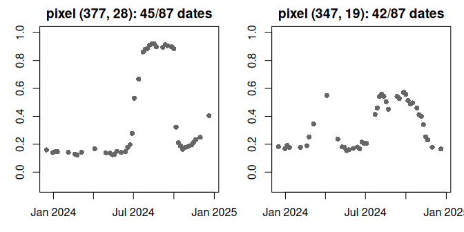
Gappy, unevenly spaced, and with residual atmosphere the mask never catches. Everything downstream is a strategy for this.
Route one: composites
The classic move is to trade time resolution for completeness.
group_by_time() splits the dataset’s slices by calendar
month; reduce_over("median") composites each group; one
collect() returns a named list, all from one graph.
monthly <- ds |>
  group_by_time("month") |>
  reduce_over("median", over = "t", nan_rm = TRUE)
mc <- collect(monthly)
names(mc)
#>  [1] "2023-12" "2024-01" "2024-02" "2024-03" "2024-04" "2024-05" "2024-06"
#>  [8] "2024-07" "2024-08" "2024-09" "2024-10" "2024-11" "2024-12"
pal <- hcl.colors(64, "Rocket")
par(mfrow = c(3, 4), mar = c(0.4, 0.4, 1.4, 0.4))
for (g in names(mc)[-1]) {                     # the twelve 2024 months
  a  <- mc[[g]]                                # (y, x, band) in dataset order
  nd <- (a[, , 2] - a[, , 1]) / (a[, , 2] + a[, , 1])
  image(t(nd[nrow(nd):1, ]), col = pal, zlim = c(-0.1, 0.9),
        axes = FALSE, main = g)
}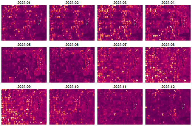
The pivots light up through July to September. But each panel is a
month smeared to one value: green-up dates, harvest dates, and
everything faster than a month are gone. (For simple within-series
patching there is also fill_gaps(), which forward-fills or
interpolates along t.)
Route two: smooth the series itself
kalman_smooth() runs a local-linear-trend Kalman filter
and smoother through every pixel’s series: a latent level and slope
evolve with small random disturbances, each observation measures the
level with noise, and missing dates simply contribute no update. The
smoother is a scan_over() body compiled through the same
machinery as every other kernel, batched over all 360k pixels at
once.
The three standard deviations are the model: sigma_lvl
and sigma_slp set how fast the level and slope may drift
between dates (smoothness), sigma_obs how noisy a single
observation is (trust). They are fixed scalars, fitted off-raster by
maximum likelihood or, as here, set by eye and judged against the data.
(For spike removal without a state-space model,
hampel_smooth() applies the classic rolling median/MAD
despike over t; it composes naturally ahead of the smoother
when residual outliers survive the masking.)
sm <- kalman_smooth(ndvi, sigma_lvl = 0.025, sigma_slp = 0.003,
                    sigma_obs = 0.07)
res <- collect(sm)          # ONE plan: both outputs share the forward
smooth <- res$mean          # filter inside a single compiled kernel
band   <- res$sd
par(mfrow = c(1, 2), mar = c(3, 3, 2, 1))
for (p in list(p1, p2)) {
  m <- smooth[p[1], p[2], ]; s <- band[p[1], p[2], ]
  plot(dates, raw[p[1], p[2], ], pch = 16, col = "grey40",
       ylim = c(-0.1, 1), xlab = "", ylab = "NDVI",
       main = glue::glue("pixel ({p[1]}, {p[2]})"))
  polygon(c(dates, rev(dates)), c(m - 2 * s, rev(m + 2 * s)),
          col = adjustcolor("firebrick", 0.15), border = NA)
  lines(dates, m, col = "firebrick", lwd = 2)
}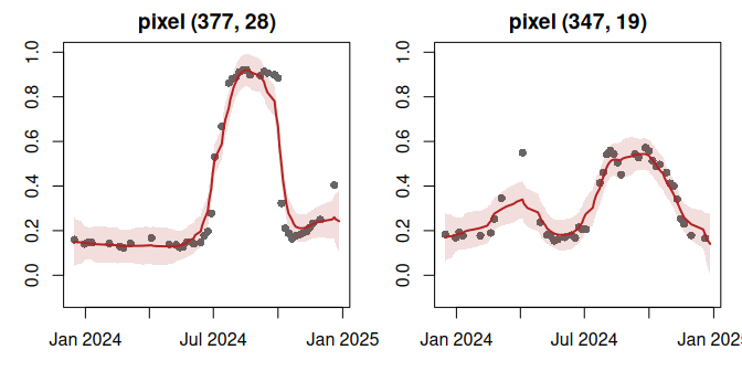
Gap-free, smooth, and dated: the pivot keeps its spring bump and its sharp summer peak, at every acquisition date, with a standard error that honestly widens where observations thin out. The smoothed cube is 98.6% complete (only pixels with fewer than three observations stay NaN).
Animate the year
gifski::save_gif(
  for (i in seq(1, length(dates), by = 2)) {
    par(mar = c(0, 0, 2, 0))
    image(t(smooth[nrow(smooth):1, , i]), col = pal, zlim = c(-0.1, 0.9),
          axes = FALSE, main = format(dates[i]))
  },
  gif_file = "figure/ndvi-timeseries.gif",
  width = 780, height = 500, delay = 0.12)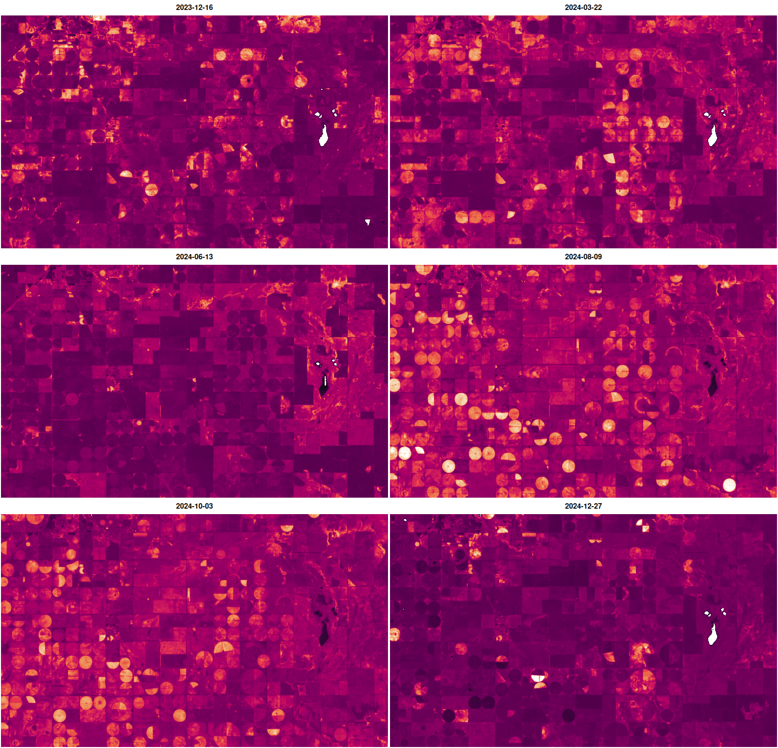
The pulsing of individual pivots is real: centre-pivot fields green up, get cut, and regrow on their own schedules, and at a ~5 day cadence the smoother keeps that signal rather than averaging it away.
Compose further: a custom temporal reducer
Everything so far returns lazy objects, so the smoothed cube is just
more graph. reduce_over() accepts a custom reducer written
in the g_* vocabulary; seasonal amplitude (how much each
pixel greens and browns over the year) is one line, and reducing the
smoothed series makes it robust to the residual outliers that
would dominate a raw max minus min:
amp <- reduce_over(sm$mean, function(x, dims)
  g_max(x, dims, nan_rm = TRUE) - g_min(x, dims, nan_rm = TRUE),
  over = "t")
preview(collect(amp), stretch = c(2, 98), main = "Seasonal NDVI amplitude")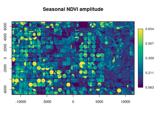
Pivots and dryland fields separate cleanly from rangeland and roads. The whole pipeline (query to phenology metric) is one graph: reads, masking, the index, an 87-step Kalman scan, and the reduction fuse and execute chunk by chunk with bounded memory.
Where to go next: the composite vignette covers the STAC-to-GeoTIFF
workflow in depth (band tables, morphological mask cleanup, streaming
writes), and scan_over() is the general primitive behind
kalman_smooth() and fill_gaps() when you want
to write your own recursive filter.