Harmonized Landsat-Sentinel composite and PCA • garry

The Harmonized Landsat Sentinel-2 (HLS) project delivers a common surface reflectance product from two sensors, giving a land observation every 2-3 days at 30 m. The two collections are spectrally harmonized but name their bands differently and carry different band sets (Landsat has thermal bands and no red edge; Sentinel-2 has red edge and a broad NIR). This vignette harmonizes both onto one band schema, builds a cloud-masked median composite, and reduces the band axis to its first three principal components. It uses the Microsoft Planetary Computer; stac_sign_mpc() signs the assets, caching the collection’s SAS token in memory and on disk until it expires.

Discover and harmonize

Query both collections over an area of interest, sign them, filter cloudy scenes, and drop duplicate acquisitions. Every step operates on the STAC items object itself (rstac’s doc_items): the filters compose on it directly, and lazy_dataset() builds the source table internally, so nothing coerces to a data frame here.

library(garry)

aoi <- c(144.24, -7.66, 144.36, -7.54)   # lon/lat bbox
mpc <- "https://planetarycomputer.microsoft.com/api/stac/v1/"

discover <- function(collection) {
  stac_query(bbox = aoi, stac_source = mpc, collection = collection,
             start_date = "2023-01-01", end_date = "2023-12-31") |>
    stac_sign_mpc() |>
    stac_filter_cloud(80) |>
    stac_drop_duplicates()
}

Each collection’s assets are mapped onto one shared schema with stac_rename_assets(): aerosol A, visible B/G/R, red edge RE1-RE3, NIR N (broad) and N2 (narrow), water vapour WV, cirrus C, SWIR S1/S2, thermal T1/T2. Unmapped assets (view angles, previews) drop out, so the map doubles as the band selector. stac_merge() unions the two harmonized item collections.

l30 <- discover("hls2-l30") |>
  stac_rename_assets(c(
    B01 = "A", B02 = "B", B03 = "G", B04 = "R", B05 = "N2", B06 = "S1",
    B07 = "S2", B09 = "C", B10 = "T1", B11 = "T2", Fmask = "Fmask"))

s30 <- discover("hls2-s30") |>
  stac_rename_assets(c(
    B01 = "A", B02 = "B", B03 = "G", B04 = "R", B05 = "RE1", B06 = "RE2",
    B07 = "RE3", B08 = "N", B8A = "N2", B09 = "WV", B10 = "C", B11 = "S1",
    B12 = "S2", Fmask = "Fmask"))

src <- stac_merge(l30, s30)
cat("bands:", paste(sort(unique(unlist(
  lapply(src$features, function(f) names(f$assets))))), collapse = " "), "\n")
#> bands: A B C Fmask G N N2 R RE1 RE2 RE3 S1 S2 T1 T2 WV

No empty-band padding or reordering is needed (unlike a VRT-based approach): lazy_dataset() gives each band only the slices that carry it, and mask() pairs a band’s slices with the matching Fmask by name. A Landsat-only thermal band and a Sentinel-only red-edge band each reduce over exactly their own observations.

Cloud-masked median composite

The reflectance and red-edge bands are read with resampling = "bilinear" onto the analysis grid; mask_asset = "Fmask" is always read nearest regardless, since interpolating packed QA bits would corrupt the flag values.

# Thermal (T1/T2) is Landsat-only and sparse, so requiring it drops most pixels
# from the PCA; keep the reflectance/red-edge bands, which both sensors provide.
bands  <- c("A", "B", "G", "R", "RE1", "RE2", "RE3", "N",
            "N2", "WV", "C", "S1", "S2")
target <- grid_from_bbox(aoi, res = 30)     # equal-area 30 m grid

garry_daemons()

comp <- lazy_dataset(
  src, grid = target, assets = bands, mask_asset = "Fmask",
  nodata = c(stats::setNames(rep(-9999, length(bands)), bands), Fmask = 255),
  resampling = "bilinear"
) |>
  mask(from = "Fmask", where = qa_bits(0:3), open = 2, dilate = 3) |>
  reduce_over("median", over = "t")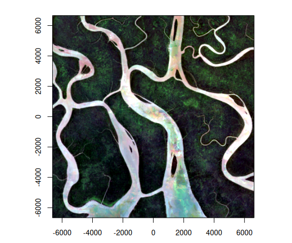

preview(comp, bands = c("R", "G", "B"))      # true-colour look (band names)

plot of chunk truecolour

PCA over the band axis

A per-pixel PCA collapses the spectral vector to a few components. Fit it in plain R on the materialized composite – fitting a model in R is perfectly reasonable; not everything belongs in the lazy graph.

cube <- stack_bands(comp)                    # LazyRaster (band, y, x)
arr  <- collect(cube)                        # (y, x, band)
px   <- matrix(arr, ncol = dim(arr)[[3]])
px   <- px[stats::complete.cases(px), , drop = FALSE]
pca  <- prcomp(px, center = TRUE, scale. = TRUE)
round(summary(pca)$importance[, 1:3], 3)     # variance explained, PC1-3
#>                          PC1   PC2   PC3
#> Standard deviation     3.204 1.242 0.905
#> Proportion of Variance 0.790 0.119 0.063
#> Cumulative Proportion  0.790 0.908 0.971

The projection onto each principal component is a linear combination of the bands – exactly reduce_over(over = "band"). band_project() builds the reducer (centre, then weight by the loading); stacking the first three gives a 3-band image. Because it is lazy, the same projection runs chunked and distributed at full resolution without ever holding the whole cube in memory.

sc  <- pca$scale                             # prcomp(scale. = TRUE): weights /= sd
pcs <- lazy_stack(
  lapply(1:3, function(i)
    reduce_over(cube, band_project(pca$rotation[, i] / sc, center = pca$center),
                over = "band")),
  along = "band")

preview(pcs)                                 # PC1-3 as R/G/B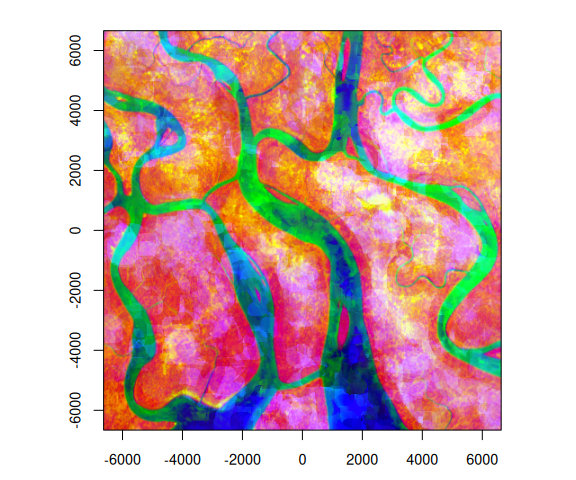

plot of chunk pca-project

The same band_project() reducer is the basis for any linear-model predict (regression, logistic, unmixing): fit in R, pass the coefficients as weights. Non-linear models (random forests, boosting) don’t trace to the compute backend – for those, collect() the composite and predict in R.