
ESA BIOMASS Level 2A products
biomass-l2a.RmdBIOMASS is ESA’s P-band synthetic aperture radar (SAR) mission. Its long wavelength sees through the canopy, which makes it a forest mission. ESA publishes three Level 2A products:
- Ground notched (GN): backscatter with the ground contribution removed, in three polarisations (HH, VH, VV), in one three-band file.
- Forest height (FH): top-of-canopy height in metres, plus a quality layer.
- Forest disturbance (FD): a change probability, an intact/disturbed classification, and a computed forest mask.
This vignette loads all three over one area of the Sangha forest, where Cameroon, the Republic of the Congo and the Central African Republic meet, and draws them. Along the way it shows authenticated reads, multi-band STAC assets, and trimming swath edges with morphology.
Authenticate
The products are open, but every request needs an ESA bearer token. Register for an EO Sign In account, then generate an offline token on the ESA MAAP portal (see the access notes on the catalogue page). The offline token lasts 90 days and exchanges for an access token that lasts 10 hours.
garry_http_auth() registers a header for every request
under a URL prefix, on this session and on every garry daemon. Passing a
function rather than a fixed header lets garry refresh the token between
runs. The header goes only to the MAAP data host, never to other servers
garry reads from.
library(garry)

maap_token <- function() {
  resp <- httr2::request(
    "https://iam.maap.eo.esa.int/realms/esa-maap/protocol/openid-connect/token"
  ) |>
    httr2::req_body_form(
      client_id = "offline-token",
      client_secret = Sys.getenv("ESA_MAAP_CLIENT_SECRET"),
      grant_type = "refresh_token",
      refresh_token = Sys.getenv("ESA_MAAP_OFFLINE_TOKEN"),
      scope = "offline_access openid"
    ) |>
    httr2::req_perform()
  httr2::resp_body_json(resp)$access_token
}

garry_http_auth(
  "https://catalog.maap.eo.esa.int/data/",
  function() paste("Authorization: Bearer", maap_token()),
  refresh = 8 * 3600
)
garry_daemons()
Find the products
All three products sit in one STAC collection,
BiomassLevel2a. Query it once and split the items by their
product:type property.
aoi <- c(14.6, 1.9, 15.0, 2.3) # lon/lat: xmin, ymin, xmax, ymax

items <- stac_query(
  aoi,
  stac_source = "https://catalog.maap.eo.esa.int/catalogue/",
  collection = "BiomassLevel2a",
  start_date = "2025-01-01",
  end_date = "2026-10-01"
)

of_type <- function(type) {
  rstac::items_filter(items, filter_fn = \(f) f$properties$`product:type` == type)
}
gn_items <- of_type("FP_GN__L2A")
fh_items <- of_type("FP_FH__L2A")
fd_items <- of_type("FP_FD__L2A")

table(vapply(items$features, \(f) f$properties$`product:type`, ""))
#>
#> FP_FD__L2A FP_FH__L2A FP_GN__L2A
#>          2          2          2
Two acquisitions cover the area, on 12 December 2025 and 14 January 2026. Every product is read onto one 100 m UTM grid, so the three line up pixel for pixel.
grid <- grid_from_bbox(aoi, res = 100, projection = "utm")Ground notched backscatter
The GN product packs its three polarisations into one file, the
enclosure_tiff asset. lazy_dataset() reads
every band of a multi-band asset as its own dataset band, and
bands names them, since the file carries no band
descriptions.
gn <- lazy_dataset(
  gn_items,
  grid,
  assets = "enclosure_tiff",
  bands = list(enclosure_tiff = c(hh = 1, vh = 2, vv = 3))
)
gn
#> ── <LazyDataset> ───────────────────────────────────────────────────────────────
#>   bands  hh vh vv
#>   time   2 slices
#>   grid   446 x 443 • f32
#>   crs    EPSG:32633
#>   graph  6 nodes • lazy
#>   ℹ plan_draw(x) to see the pipeline
GN values are linear backscatter intensity. Average the two acquisitions in linear units, convert to decibels, and draw HH, VH and VV as red, green and blue.
to_db <- function(x) {
  x |>
    reduce_over("mean", over = "t") |>
    lazy_map(fn = \(v) 10 * log10(v))
}

preview(to_db(gn), bands = c("hh", "vh", "vv"), main = "GN, as read")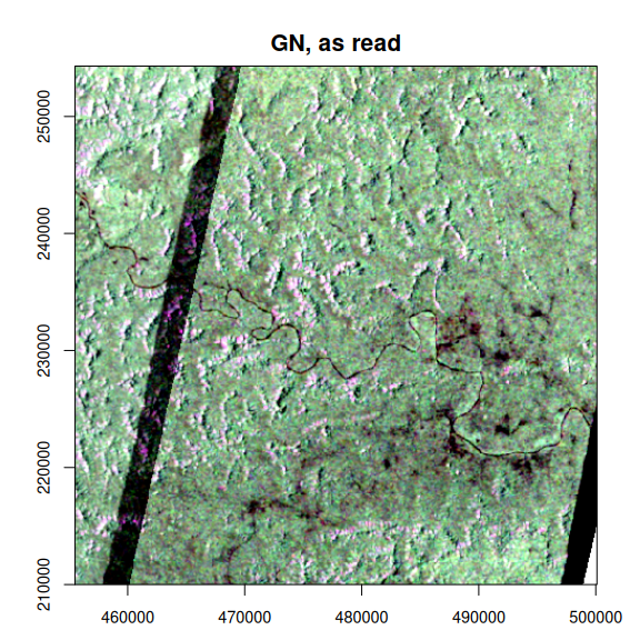
The dark diagonal stripe is an artefact. Each product fills the edge of its radar swath with exact zeros rather than its declared nodata value, so the mean drags in zeros wherever the two swaths overlap. Treating zeros as nodata removes the stripe but leaves a thin seam: the last pixel or two inside each swath are low but not zero.
Trimming the seam is morphology. shrink_footprint()
erodes each slice’s valid footprint by a few pixels, the counterpart of
the dilate argument of apply_mask(), which
grows a mask. boundary = "keep" erodes only real nodata
edges and leaves the border of the analysis grid alone. The panels below
zoom in on the seam.
clean <- function(x) {
  x |>
    lazy_map(fn = \(v) g_ifelse(v > 0, v, NaN)) |>
    shrink_footprint(radius = 2, boundary = "keep")
}

zoom <- grid_spec(grid_crs(grid), extent = c(455500, 226000, 471500, 242000),
                  res = 100)
gn_zoom <- lazy_dataset(gn_items, zoom, assets = "enclosure_tiff",
                        bands = list(enclosure_tiff = c(hh = 1, vh = 2, vv = 3)))
zeros_out <- lazy_map(gn_zoom, fn = \(v) g_ifelse(v > 0, v, NaN))

op <- par(mfrow = c(1, 3), mar = c(1, 1, 2, 1))
preview(to_db(gn_zoom), bands = c("hh", "vh", "vv"), main = "as read",
        axes = FALSE)
preview(to_db(zeros_out), bands = c("hh", "vh", "vv"), main = "zeros removed",
        axes = FALSE)
preview(to_db(clean(gn_zoom)), bands = c("hh", "vh", "vv"),
        main = "footprint shrunk by 2 px", axes = FALSE)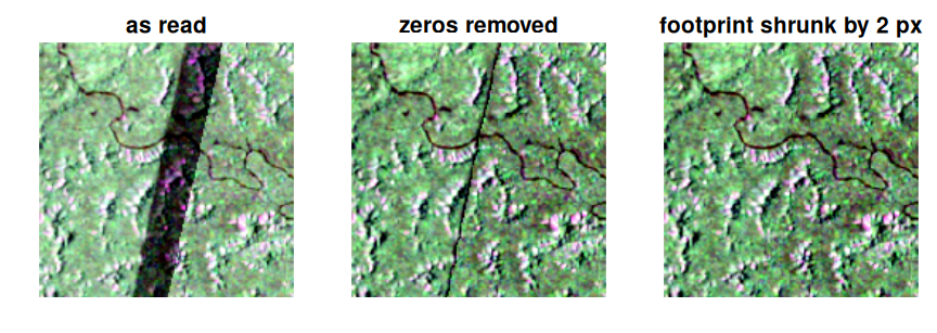
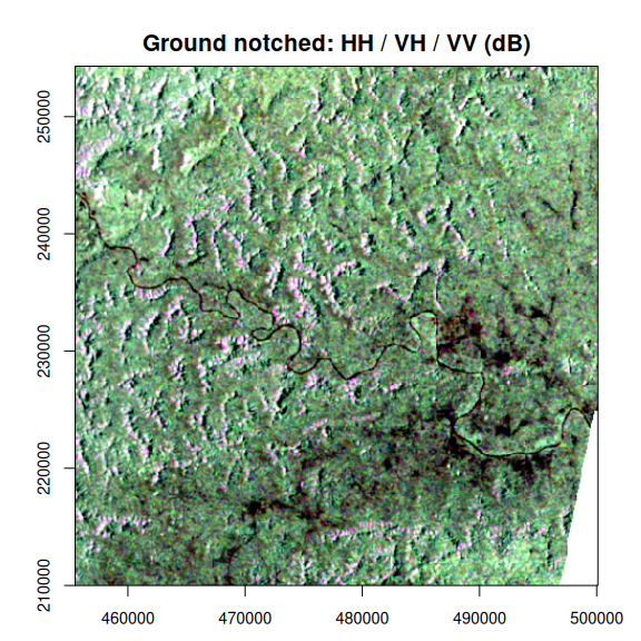
par(op)With the edges cleaned, the composite shows the Sangha river and its tributaries as dark lines, terrain relief from slopes facing towards and away from the radar, and dark open patches along the river in the east of the area.
Forest height
Forest height and its quality layer are separate single-band assets.
Renaming through bands gives the height a readable name,
and the same cleaning applies.
height <- lazy_dataset(
  fh_items,
  grid,
  assets = "enclosure_i_fh_tiff",
  bands = list(enclosure_i_fh_tiff = c(height = 1))
) |>
  clean() |>
  reduce_over("mean", over = "t")

preview(height, main = "Forest height (m)",
        col = grDevices::hcl.colors(64, "YlGn", rev = TRUE))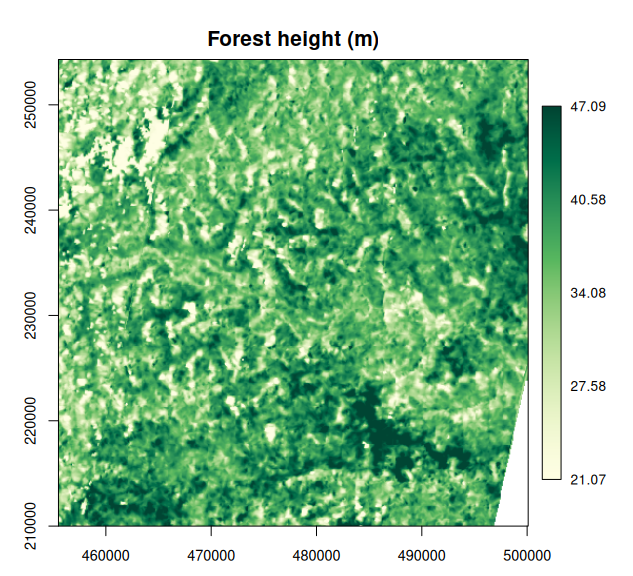
Forest disturbance
The FD product has three layers. In this first release, the disturbance probability and classification hold no valid pixels here; a valid-pixel count over both acquisitions shows it. Only the computed forest mask is populated.
fd <- lazy_dataset(
  fd_items,
  grid,
  assets = c("enclosure_i_probability_tiff", "enclosure_i_fd_tiff",
             "enclosure_i_cfm_tiff"),
  bands = list(
    enclosure_i_probability_tiff = c(probability = 1),
    enclosure_i_fd_tiff = c(disturbed = 1),
    enclosure_i_cfm_tiff = c(forest = 1)
  )
)
valid <- collect(reduce_over(fd, "count", over = "t"))
stats::setNames(apply(valid, 3, sum), names(fd))
#> probability   disturbed      forest
#>           0           0      309657
The mask is 1 for forest and 0 for non-forest. Taking the minimum over the two acquisitions keeps pixels that are forest in both.
forest <- reduce_over(fd[["forest"]], "min", over = "t")
preview(forest, main = "Computed forest mask", stretch = NULL,
        col = c("#d9cba3", "#1b5e20"), legend = FALSE)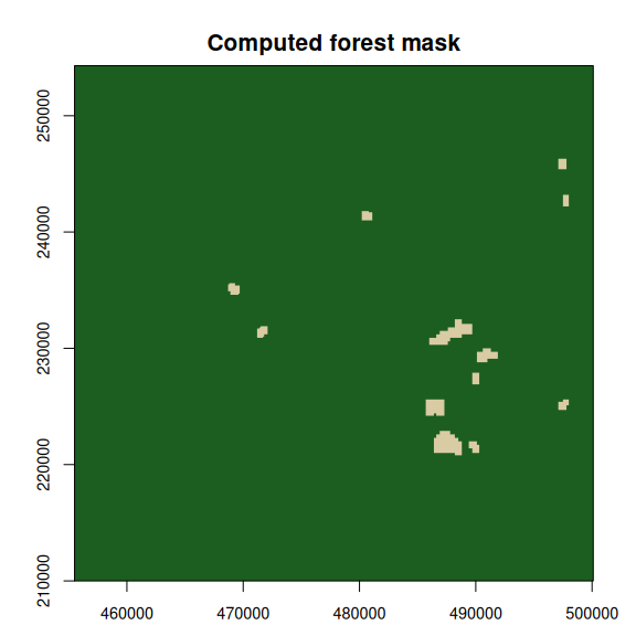
The non-forest patches match the dark open areas along the river in the backscatter composite.