Reading Alpha Earth embeddings

Alpha Earth Foundations (AEF) by Google is published by Source Cooperative. This dataset is a collection of annual geospatial embeddings stored as 64-band Int8 Cloud-Optimised GeoTIFFs: each band is one dimension of a learned embedding, quantised to a signed byte and decoded with a nonlinear, sign-preserving transform, ((x / 127.5)^2) * sign(x).

A multi-band file is just another source: give lazy_dataset() the path and it builds one band per file band, named from the file’s band descriptions (A00 .. A63 here). Each band is its own source, so at collect() the reads fan out band-by-band across the reader pool – many connections issuing range requests concurrently, which is what makes a 64-band remote read fast. This vignette reads one tile, resamples to 30 m, dequantises on the read, and renders three arbitrary bands as a false-colour composite.

Read and dequantise

library(garry)

# One AEF annual tile (Source Cooperative, public, no auth). UTM 36S, ~10 m.
tile <- paste0("https://data.source.coop/tge-labs/aef/v1/annual/2021/36S/",
               "xekh5rjs4wg6wb9b4-0000000000-0000000000.tiff")

# the analysis grid: the tile's own footprint at 30 m
grid <- grid_from_src(tile, 30)

embeddings <- lazy_dataset(tile, grid, resampling = "average") |>
  lazy_map(fn = dequantize_aef, dtype = "f32")

embeddings
#> ── <LazyDataset> ────────────────────────────────
#>   bands  A00 A01 A02 A03 A04 A05 A06 A07 A08 A09 A10 A11 A12 A13 A14 A15 A16 A17 A18 A19 A20 A21 A22 A23 A24 A25 A26 A27 A28 A29 A30 A31 A32 A33 A34 A35 A36 A37 A38 A39 A40 A41 A42 A43 A44 A45 A46 A47 A48 A49 A50 A51 A52 A53 A54 A55 A56 A57 A58 A59 A60 A61 A62 A63
#>   time   1 slice
#>   grid   2732 x 2731 • f32
#>   crs    EPSG:32736
#>   graph  192 nodes • lazy
#>   ℹ draw(x) to see the pipeline

lazy_dataset() records a lazy 64-band dataset; nothing is fetched yet (the construction costs one metadata probe, however many bands the file carries). dequantize_aef() is applied as a map, which garry fuses onto the read so the nonlinear decode runs on-device, not as a separate pass.

Collect three bands and plot

Pick three arbitrary embedding dimensions and collect just those: the band-axis subset means only those three are ever read or computed or preview a coarser overview of the tile to take a quick look.

garry_daemons()
# cube <- collect(embeddings[c("A09", "A10", "A11")])

preview(embeddings[c("A09", "A10", "A11")], bands=c(2,1,3))   # False-colour composite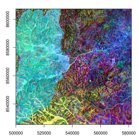

plot of chunk aef-plot

Neighbouring pixels of similar land cover carry similar embeddings, so the false-colour image segments the landscape into coherent regions: the structure the embeddings encode. But three bands show three of sixty-four dimensions. The clustering below uses all of them.

Cluster the full embedding space

An unsupervised k-means over the 64-dimensional embedding vectors segments the landscape without a single training label. The pattern is fit-small, predict-lazily – and neither half needs the raster on disk:

Materialise once. Both halves below read all 64 bands, so decode the tile a single time into a local cube and work from that. This is the one expensive step, and it is explicit: the remote fetch and the dequant happen once, and everything after reads local pixels.

cube <- materialise(embeddings)   # pass dir= to keep it beyond the session

Fit. k-means needs pixels in R, but not all 7.5 million of them – 100k scattered ones place five centroids perfectly well. extract_points() reads just those, straight out of the cube: GDAL touches only the blocks holding points, so this costs a fraction of a second rather than another pass over the raster.

Points are a wk xy vector carrying their own CRS, so they are placed on the grid explicitly rather than by assumption (wk::as_xy() converts points from sf, terra or a data frame).

set.seed(42)
n   <- 1e5
pts <- wk::xy(
  stats::runif(n, xmin(grid), xmax(grid)),
  stats::runif(n, ymin(grid), ymax(grid)),
  crs = grid@crs
)

px <- extract_points(cube, pts)              # (100000, 64)
dim(px)
#> [1] 100000     64
px <- px[stats::complete.cases(px), ]
km <- kmeans(px, centers = 5)
km$size
#> [1] 12935 30046 24230 22641 10148

The same call is how a model gets its training table off any garry pipeline: give it the GEDI shots, the field plots or the labelled points instead of random ones. interp = "bilinear" interpolates the four surrounding cell centres for continuous data measured off-grid, and krnl_dim reads a window around each point instead of a single cell.

Assign. Every 30 m pixel goes to its nearest centroid: argmax_k (x . c_k - |c_k|^2 / 2), and x . c_k is a linear combination of bands – the band_project() reducer from the PCA article. The argmax is expressible in the same public vocabulary, so the WHOLE assignment runs inside the graph: a custom band reducer composes six projections with a comparison chain, and collect() returns the finished cluster map. This is ordinary user code – garry’s shipped verbs are built from exactly these pieces, with no privileged access to the engine.

nearest_center <- function(centers) {
  ct   <- unname(as.matrix(centers))            # k x band
  half <- rowSums(ct^2) / 2
  proj <- lapply(seq_len(nrow(ct)), function(k) band_project(ct[k, ]))
  function(x, dims) {
    s1   <- proj[[1]](x, dims) - half[[1]]      # score against centre 1
    best <- s1
    cl   <- s1 * 0 + 1                          # current best label
    for (k in 2:nrow(ct)) {
      sk   <- proj[[k]](x, dims) - half[[k]]
      hit  <- sk > best
      cl   <- g_ifelse(hit, k, cl)
      best <- g_ifelse(hit, sk, best)
    }
    g_ifelse(g_is_nodata(s1), NaN, cl)          # nodata stays nodata
  }
}

clusters <- reduce_over(stack_bands(cube),
                        nearest_center(km$centers), over = "band")
clmap <- collect(clusters)

garry_daemons(0, 0)

One fused kernel reads the 64-band cube once, computes every projection and the argmax per pixel, and only the finished single-band cluster map ever reaches R. (Want the raw scores instead? Stack plain band_project() reducers with lazy_stack(along = "band") and take max.col() host-side – same digital numbers.)

The k-means prediction can also stream straight to disk. Note the dtype and overview_resampling arguments: COG overviews default to “average”, and an averaged class label is meaningless, so categorical outputs want “nearest”:

write_tif(
  clusters,
  "km-aef.tif",
  dtype = "i16",
  cog = TRUE,
  overview_resampling = "nearest"
)

And the final k-means map:

preview(
  clmap,
  col = c("#E41A1C", "#377EB8", "#4DAF4A", "#984EA3", "#FF7F00")
)

plot of chunk km-plot

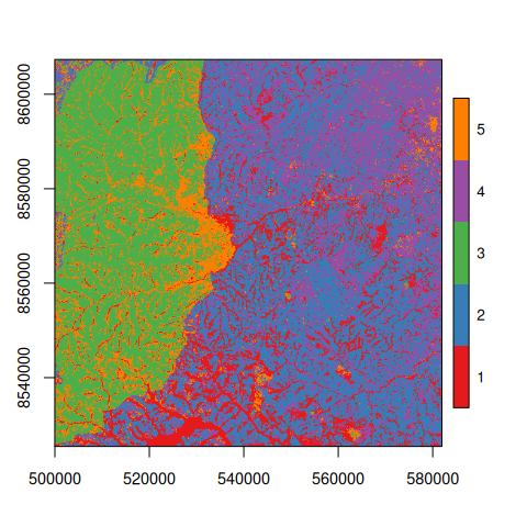
Five clusters, no labels, and the landscape decomposes into its structure: the dendritic drainage network, the river corridor and settlement strip, and the textured forest mosaic each claim their own class. The same dequantised dataset feeds any downstream verb the same way – a band-axis PCA, a similarity search, or a classifier fit on the collected array.