Getting started with garry • garry

garry is a lazy raster engine. Verbs like lazy_source(), focal(), and reduce_over() do not compute anything; each one adds a node to an intermediate representation (IR) graph, and the whole graph runs only when you call collect(). At that point garry plans the computation, splits it into chunks, fuses adjacent operations into single compiled kernels (via anvl, which lowers to XLA), and executes them with bounded memory. GDAL handles all reading, warping, and writing; the compute vocabulary is a small closed set of primitives (map, focal, reduce, scan, warp, stack) that compose freely.

This vignette walks the core loop on a single elevation tile: open lazily, build a pipeline, inspect the graph, execute. The tile is Mount Hood, Oregon (LANDFIRE elevation, 30 m, UTM zone 10N), read straight from GitHub over HTTP; nothing is downloaded until execution touches it.

Open a raster lazily

library(garry)

f <- paste0("/vsicurl/https://raw.githubusercontent.com/",
            "firelab/gdalraster/main/sample-data/",
            "lf_elev_220_mt_hood_utm.tif")
el <- lazy_source(f)
el
#> ── <LazyRaster> source  1013×799 f32 ───────────────────────────────────────────
#>   grid   1013 x 799 • f32
#>   crs    EPSG:26910
#>   graph  1 nodes • lazy
#>   ℹ draw(x) to see the pipeline

Opening reads only metadata: one HTTP request for the file header, zero pixels. The LazyRaster knows its grid (extent, resolution, CRS, dtype) and carries a one-node graph. Accessors read the grid without touching the file again:

res(el)
#> [1] 30 30
c(xmin(el), ymin(el), xmax(el), ymax(el))
#> [1]  587049.6 5013342.4  617439.6 5037312.4

preview(el, main = "Mount Hood elevation (m)")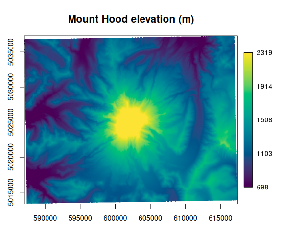

plot of chunk hood-preview

preview() is the cheap look: it renders a decimated version sized to your device, not the full raster.

Build a computation

Arithmetic on a LazyRaster returns a new LazyRaster; nothing runs.

el_km <- el / 1000
el_km
#> ── <LazyRaster> map ────────────────────────────────────────────────────────────
#>   grid   1013 x 799 • f32
#>   crs    EPSG:26910
#>   graph  2 nodes • lazy
#>   ℹ draw(x) to see the pipeline

focal() applies a moving-window (stencil) operation. Its fn receives a list of the (2r + 1)^2 shifted copies of the window, ordered row-major over (dy, dx) offsets, and processes the whole neighbourhood vectorised across every pixel at once. A 3x3 mean is one line:

sm <- focal(el, radius = 1L, fn = function(sh) Reduce(`+`, sh) / 9)

The same convention supports real terrain analysis. For a radius-1 stencil the list indexes as a 3x3 grid: sh[[2]] is the neighbour to the north, sh[[8]] south, sh[[4]] west, sh[[6]] east, sh[[5]] the centre. Central differences over those four neighbours give the elevation gradient, the gradient gives the surface normal, and the dot product with a sun vector is a hillshade:

hillshade <- function(elev, azimuth = 315, altitude = 45) {
  rs  <- res(elev)
  az  <- (90 - azimuth) * pi / 180
  alt <- altitude * pi / 180
  sun <- c(cos(alt) * cos(az), cos(alt) * sin(az), sin(alt))
  focal(elev, radius = 1L, fn = function(sh) {
    dzdx <- (sh[[6]] - sh[[4]]) / (2 * rs[[1]])   # east - west
    dzdy <- (sh[[2]] - sh[[8]]) / (2 * rs[[2]])   # north - south
    v <- (-dzdx * sun[[1]] - dzdy * sun[[2]] + sun[[3]]) /
      sqrt(dzdx^2 + dzdy^2 + 1)
    g_ifelse(v < 0, 0, v)                         # clamp shadowed slopes
  })
}

hs <- hillshade(el)

The body mixes ordinary arithmetic with g_ifelse(), one of the g_* functions garry’s kernels are written in. The same closure runs in two worlds: as plain R on matrices (the testing oracle) and traced through anvl into a compiled XLA kernel (execution). You never choose; garry does.

The graph is the object

draw(hs)
#> ── <LazyRaster> 1013 x 799 • f32 ───────────────────────────────────────────────
#> ◫ focal  r=1
#> └─ ◈ source  1013×799 f32

That is the whole mental model: hs is this pipeline, not an array. When it executes, the planner will fuse the focal into its source read, compile its body once, and run it chunk by chunk.

Grids are strict

Every LazyRaster is pinned to its grid, and binary operations refuse operands whose grids differ; there is no silent resampling. Build a coarser 270 m grid and aggregate onto it with align():

coarse <- grid_spec(crs = "EPSG:26910",
                    extent = c(xmin(el), ymin(el), xmax(el), ymax(el)),
                    res = 270)
el_mean <- align(el, coarse, resampling = "average")

Mixing the two grids is an error, and the error is a feature: an analysis that silently warps one operand is an analysis with an undisclosed resampling step.

el - el_mean
#> Error in `.lazy_binop()`:
#> ! grids differ (resolution differs: 30 x 30 vs 270 x 270); use `align(a,
#>   b, to = ...)` first

State the resample explicitly and it composes like anything else. Aligning the same source twice, once point-sampled and once aggregated, and differencing on the shared grid gives a local relief model: elevation relative to the neighbourhood mean.

el_pt  <- align(el, coarse, resampling = "bilinear")
relief <- el_pt - el_mean
preview(relief, main = "Local relief (m)")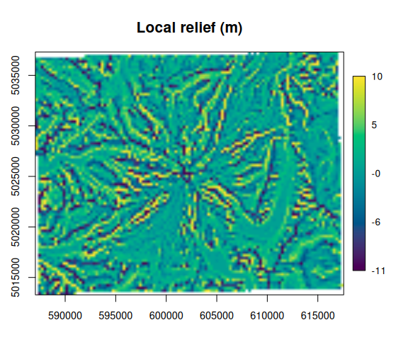

plot of chunk hood-relief

One v1 rule to know: align() applies to sources, not to computed results (warping a computed raster raises an error suggesting the alternatives). Align inputs onto the analysis grid first, then compute; or materialise a result with write_tif() and re-open it.

Execute

collect() runs the graph and returns an ordinary array carrying a gis attribute (extent, CRS) so the result stays georeferenced:

arr <- collect(hs)
str(attr(arr, "gis"))
#> List of 5
#>  $ type    : chr "raster"
#>  $ bbox    : num [1:4] 587050 5013342 617440 5037312
#>  $ dim     : int [1:3] 1013 799 1
#>  $ srs     : chr "PROJCS[\"NAD83 / UTM zone 10N\",GEOGCS[\"NAD83\",DATUM[\"North_American_Datum_1983\",SPHEROID[\"GRS 1980\",6378"| __truncated__
#>  $ datatype: chr "Float32"
preview(arr, col = grDevices::hcl.colors(64, "Rocket"),
        legend = FALSE, main = "Hillshade")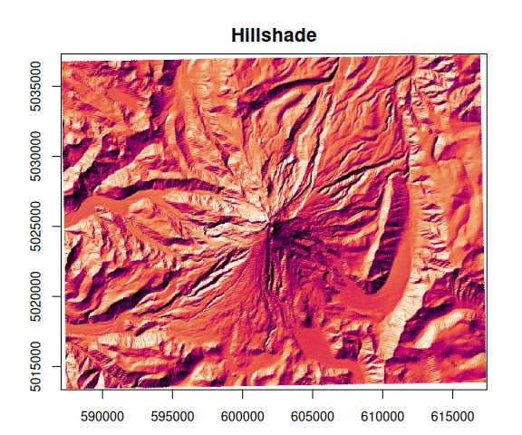

plot of chunk hood-collect

Write straight to a GeoTIFF instead with write_tif(); chunks stream to disk as they finish, so the full result never needs to fit in memory:

tif <- file.path(tempdir(), "hood-hillshade.tif")
write_tif(hs, tif)
file.size(tif)
#> [1] 1673358

For handoff to the wider R spatial ecosystem, as_terra() converts a collected array into a terra::SpatRaster.

Where this scales

Everything above ran in a single R process, which is exactly right at this size. The same collect() call distributes across daemon pools (garry_daemons()) with separate read and compute fleets, warp-on-read onto an analysis grid, and memory-bounded scheduling; that machinery is the subject of the next vignette, which builds a cloud-masked satellite composite from a STAC catalogue.