OlmoEarth embeddings from Zarr • garry

OlmoEarth v1.3 from Ai2 summarises each year of Sentinel-1, Sentinel-2 and Landsat 8/9 imagery as a 128-dimensional vector per 10 m pixel. The embeddings are public on Source Cooperative as one Zarr v3 store, with no account or signing needed:

one group per UTM zone (utm01 to utm60), each holding an embeddings array with axes (time, band, y, x);
nine years, 2017 to 2025 (2023 to 2025 are global, earlier years are being backfilled);
Int8 codes, decoded by sign(q) * (|q| / 127.5)^2, with -128 as nodata;
the first 64 dimensions form a complete embedding on their own (Matryoshka training) and are stored in their own chunks.

This vignette reads two years over Jasper National Park, Alberta, where a wildfire burned about 33,000 ha in July 2024, and maps how far each pixel’s embedding moved between 2023 and 2025.

Open the store

GDAL’s Zarr driver reads the store directly. A ZARR: connection string names the zone group and the array; garry adds the /vsicurl/ prefix to a bare https store, as it does for any URL.

library(garry)

store <- "https://data.source.coop/olmoearth/olmoearth-v1-3-embeddings/embeddings.zarr"
src <- paste0('ZARR:"', store, '/utm11":/embeddings')

Each zone is in its own UTM CRS (Jasper is in zone 11, EPSG:32611), on a 10 m grid anchored at the zone origin. A grid in that CRS at 10 m with edges on multiples of 10 m is a plain window of the array, so the read needs no resampling. Edges on multiples of 2560 m also line up with the store’s 256-pixel chunks, so every chunk fetched is used in full.

grid <- grid_spec("EPSG:32611", c(417280, 5834240, 445440, 5870080), res = 10)
dim(grid)
#>    y    x 
#> 3584 2816

lazy_dataset() reads the array’s dimension tags (GDAL flattens (time, band) into classic bands and labels each one) and lays the array out as dataset bands by year. bands = 1:64 keeps the 64-dimension embedding, which halves the bytes read.

oe <- lazy_dataset(src, grid, bands = 1:64)
oe
#> ── <LazyDataset> ───────────────────────────────────────────────────────────────
#>   bands  b1 b2 b3 b4 b5 b6 b7 b8 ... (+56)
#>   time   9 slices
#>   grid   2816 x 3584 • f32
#>   crs    EPSG:32611
#>   graph  1152 nodes • lazy
#>   ℹ plan_draw(x) to see the pipeline
time_labels(oe)
#> [1] "2017" "2018" "2019" "2020" "2021" "2022" "2023" "2024" "2025"

Nothing has been fetched yet beyond the store’s metadata.

Read two years

time_sel() picks a year, dequantize_olmoearth() decodes the Int8 codes (the nodata code is already NaN, so it stays NaN), and stack_bands() turns the year into one (band, y, x) cube.

year <- function(y) {
  time_sel(oe, y) |>
    lazy_map(fn = dequantize_olmoearth, dtype = "f32") |>
    stack_bands()
}

Both years feed every step below, so fetch them once into local cubes. materialise() runs both in one execution. The store’s chunks hold 64 bands each, and garry reads all 64 bands of a window in one task, so every chunk crosses the network once.

garry_daemons()
t0 <- Sys.time()
cubes <- materialise(list(y2023 = year("2023"), y2025 = year("2025")))
Sys.time() - t0
#> Time difference of 1.33462 mins

False colour

A principal component analysis of the 64 dimensions gives a false-colour image. Fit it on a sample of 2025 pixels, then project every pixel of both years with band_project() so the colours mean the same thing in each.

fit_pca <- function(cube, grid, n = 2e4) {
  bb <- grid_bbox(grid)
  pts <- wk::xy(
    stats::runif(n, bb[["xmin"]], bb[["xmax"]]),
    stats::runif(n, bb[["ymin"]], bb[["ymax"]]),
    crs = grid_crs(grid)
  )
  px <- extract_points(cube, pts)
  prcomp(px[stats::complete.cases(px), ])
}

false_colour <- function(cube, pca) {
  lazy_stack(lapply(1:3, function(k) {
    reduce_over(cube, band_project(pca$rotation[, k], center = pca$center),
                over = "band")
  }), along = "band")
}

set.seed(1)
pca <- fit_pca(cubes$y2025, grid)
summary(pca)$importance[, 1:3]
#>                              PC1      PC2       PC3
#> Standard deviation     0.9810468 0.562912 0.4375965
#> Proportion of Variance 0.4393300 0.144640 0.0874100
#> Cumulative Proportion  0.4393300 0.583970 0.6713800

op <- par(mfrow = c(1, 2))
preview(false_colour(cubes$y2023, pca), main = "2023")
preview(false_colour(cubes$y2025, pca), main = "2025")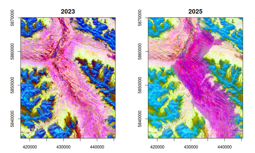

plot of chunk false-colour

par(op)

The burned valley floor turns magenta in 2025. The alpine slopes shift colour too: snow and growing seasons differ between years, and the embeddings record that. The next section measures which shift is larger.

Map the change

The cosine distance 1 - (a . b) / (|a| |b|) between a pixel’s 2023 and 2025 vectors measures how much its embedding changed, whatever the cause. The vectors are not unit length, so the norms stay in the formula. Each term is a band reduction, and garry fuses the whole expression into one kernel over the two cubes.

a <- cubes$y2023
b <- cubes$y2025
dot <- reduce_over(a * b, "sum", "band")
cos_dist <- 1 - dot / sqrt(reduce_over(a * a, "sum", "band") *
                           reduce_over(b * b, "sum", "band"))
change <- collect(cos_dist)
summary(as.vector(change))
#>     Min.  1st Qu.   Median     Mean  3rd Qu.     Max. 
#> 0.003924 0.015897 0.023107 0.064542 0.101952 0.493835

preview(change, col = grDevices::hcl.colors(64, "Inferno"),
        main = "Cosine distance, 2023 to 2025")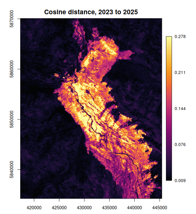

plot of chunk change-map

The burn scar stands out at roughly ten times the distance of the unburned forest and alpine terrain around it, with the Athabasca River, its lakes and unburned stands inside the perimeter staying dark. No labels and no imagery went into the map: only two years of embeddings.

A threshold turns the map into an area. The value is a choice rather than a calibration; on this map it sits in the gap between the two modes of the distribution.

moved <- sum(change > 0.1, na.rm = TRUE) * 100 / 1e4 # 10 m pixels to ha
round(moved)
#> [1] 25446

Across zones

Each zone is a separate array in its own CRS, so an area across a zone boundary reads from both. Give lazy_dataset() every zone’s array and a grid in any CRS: the warper reprojects each zone into every window and mosaics them, still reading all of a year’s bands in one task. Greenwich, on the meridian between zones 30 and 31, on the British National Grid:

zones <- paste0('ZARR:"', store, "/utm", c(30, 31), '":/embeddings')
london <- grid_spec("EPSG:27700", c(528900, 172400, 548900, 182400), res = 10)

greenwich <- lazy_dataset(zones, london, bands = 1:64) |>
  time_sel("2025") |>
  lazy_map(fn = dequantize_olmoearth, dtype = "f32") |>
  stack_bands() |>
  materialise()

set.seed(1)
pca_london <- fit_pca(greenwich, london)

preview(false_colour(greenwich, pca_london), main = "Greenwich, 2025")
lines(gdalraster::transform_xy(cbind(0, seq(51.4, 51.6, by = 0.01)),
                               "EPSG:4326", "EPSG:27700"),
      col = "white", lty = 2)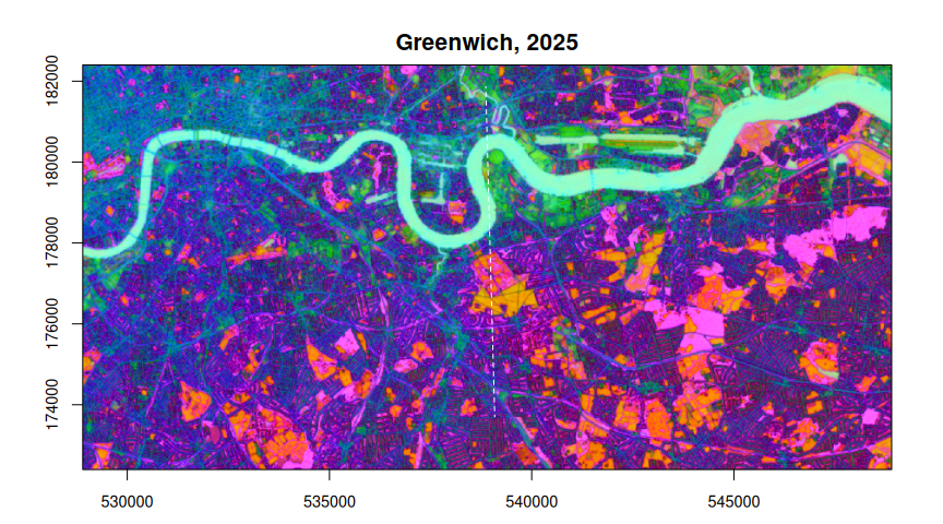

plot of chunk zones-map

The dashed line is the meridian. Each zone carries embeddings a little past its own meridian, so near the boundary both zones hold a vector for the same pixel, and the later zone in zones wins. How far apart are the two? Read each zone alone and take the cosine distance where both have data:

zone <- function(z) {
  lazy_dataset(z, london, bands = 1:64) |>
    time_sel("2025") |>
    lazy_map(fn = dequantize_olmoearth, dtype = "f32") |>
    stack_bands()
}
z30 <- zone(zones[1])
z31 <- zone(zones[2])
gap <- collect(1 - reduce_over(z30 * z31, "sum", "band") /
  sqrt(reduce_over(z30 * z30, "sum", "band") *
       reduce_over(z31 * z31, "sum", "band")))
mean(!is.na(gap))         # share of the area both zones cover
#> [1] 0.672939
median(gap, na.rm = TRUE) # their median cosine distance there
#> [1] 0.02144197
garry_daemons(0, 0)

Both zones cover 67% of this area, and there their vectors sit a median cosine distance of 0.021 apart: they were computed in different projections, but the difference is the size of the year-to-year change in unburned ground at Jasper, and the join does not show.

Notes

Southern zones use the northern CRS, so their northings are negative. GDAL and garry handle this as any other coordinate.
Dimensions. Use 64 or 128 dimensions throughout an analysis, never a
1. Reading all 128 (bands = 1:128) doubles the bytes.
Similarity. For cosine similarity as a dot product, normalise the vectors first; their norms run from about 3.0 to 3.8.
Window seams. The embeddings were computed in independent 2048 x 2048 pixel windows, and their edges can show as faint straight lines in derived maps: the vertical line at x = 430,080 m in the change map is one (the step between neighbouring columns is about seven times its usual size there).