Distances and neighbours • shoal

Every clustering algorithm rests on a notion of how far apart two rows are. shoal exposes that layer directly through two functions. shoal_dist() computes every pairwise distance and returns R’s own dist class. shoal_knn() finds each row’s k nearest neighbours and returns their indices and distances. Both take the same nine metrics and agree with each other to the last bit.

The calls are simple. The decisions around them are not, and this vignette is organised around four of them: which metric, a full matrix or neighbours only, a tree or a scan, and what to build from a neighbour result once you have one.

library(shoal)
x <- as.matrix(iris[, 1:4])

Which metric

Metric	Measures	Reach for it when
`euclidean`	Straight-line distance.	Columns are on comparable scales. The default, and what k-means assumes.
`manhattan`	Sum of absolute differences.	Outlying values in one column should not dominate.
`maximum`	Largest single difference.	One column out of tolerance is what matters.
`minkowski`	The family that contains the three above, with power `p`.	You want something between Manhattan and Euclidean.
`canberra`	Absolute differences relative to magnitude.	Counts and abundances, where a difference of 1 means more near zero.
`binary`	Fraction of positions where exactly one row is non-zero.	Presence and absence data.
`cosine`	One minus the cosine of the angle between the rows.	Direction matters and magnitude does not: embeddings, term counts.
`correlation`	One minus the Pearson correlation across the columns.	Profiles should match in shape regardless of level or scale.
`mahalanobis`	Euclidean distance after decorrelating and scaling the columns.	Columns are correlated or on different scales and you want each to count once.

The metrics shared with stats::dist() follow its definitions exactly, including the way Canberra drops degenerate terms and the fact that its denominator is |x| + |y| as the C code computes it, not the |x + y| its documentation states. Cosine is correlation without centring each row on its own mean, so the two agree on rows that already average zero.

A simple check of what a metric does is to ask how often a row’s nearest neighbours share its label. On iris, most metrics agree with the species about 95 percent of the time.

species <- iris$Species
agreement <- function(metric) {
  nn <- shoal_knn(x, k = 5L, metric = metric)
  mean(species[nn$id] == species[row(nn$id)])
}
sapply(c("euclidean", "manhattan", "cosine", "correlation", "mahalanobis"),
       agreement)
#>   euclidean   manhattan      cosine correlation mahalanobis 
#>   0.9480000   0.9466667   0.9573333   0.9480000   0.8613333

Mahalanobis does worse, and the reason is instructive. It whitens with the covariance of the whole sample, and in iris the largest correlated direction, petal length against petal width, is also the direction that separates the species. Whitening on the pooled covariance shrinks exactly the axis that carries the signal. Mahalanobis is the right choice when the correlation is within-group structure you want to discount, not between-group structure you want to find. Pass cov to whiten with a covariance estimated from a single group, or from a reference sample, and that problem goes away.

A full matrix or neighbours only

A distance matrix holds every pair, which is n (n - 1) / 2 numbers. A neighbour search holds k per row. The difference is not a constant factor; it is the difference between quadratic and linear.

d <- shoal_dist(x)
nn <- shoal_knn(x, k = 10L)
object.size(d)
#> 90800 bytes
object.size(nn$dist) + object.size(nn$id)
#> 20256 bytes

At 150 rows both are trivial. At 50,000 rows the matrix is 9.3 GB and the neighbours are under 6 MB. At a million rows the matrix does not exist, and the neighbours are a search of a few seconds.

Reach for the matrix when a consumer needs every pair: shoal_hclust(), shoal_silhouette(), cmdscale(), cluster::pam(). Even then, if the matrix is only a stepping stone to a dendrogram, pass the raw data to shoal_hclust() instead; it writes the distances straight into the buffer the clustering consumes and never holds a second copy. Reach for neighbours for everything else.

The two functions share every convention that can be shared. Rows with missing or non-finite values are dropped by shoal_dist(), with a warning, and refused by shoal_knn(), because dropping rows would renumber the indices it returns. Ties in a neighbour search are broken by row index, so a result is fully determined by its input.

A tree or a scan

shoal_knn() has two exact search algorithms behind it. A kd-tree partitions space and skips regions that cannot hold a nearer point. A scan compares every pair in parallel. Both return identical results, tie order included, so the choice is purely about speed, and the rule is dimension. A tree prunes well in a few dimensions and hardly at all beyond about ten, where the scan is several times faster than any tree. The default search = "auto" takes the tree up to 8 columns and the scan beyond.

tree <- shoal_knn(x, k = 5L, search = "kdtree")
scan <- shoal_knn(x, k = 5L, search = "brute")
identical(tree$id, scan$id) && identical(tree$dist, scan$dist)
#> [1] TRUE

The tree serves every metric except Canberra and binary, whose distances no rectangle can bound. Cosine and correlation go through a normalised copy of the rows, on which Euclidean distance orders points exactly as the metric does, while the distances reported are still the metric itself. Force search = "brute" when you know the data is wide, or search = "kdtree" when it is narrow but has more than 8 columns and you want to check for yourself.

What to build from neighbours

A neighbour result is a small, regular structure: id and dist, one row per point, nearest first. Several things the package does not do itself are a few lines from it.

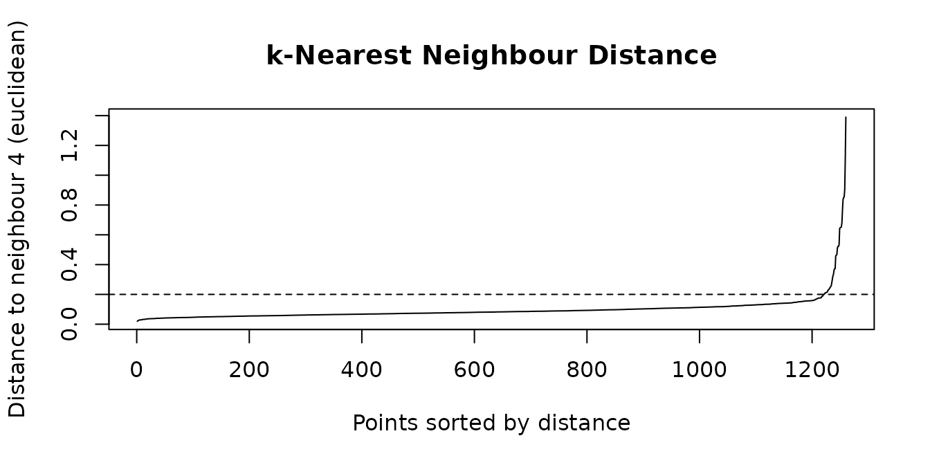
The radius for DBSCAN

Each point’s distance to its k-th neighbour, sorted, has an elbow where the dense points end and the sparse ones begin. That elbow is eps, with min_samples = k + 1 because DBSCAN counts the point itself. The plot() method draws it; vignette("shoal") walks through the choice on the rings data.

plot(shoal_knn(rings, k = 4L))
abline(h = 0.2, lty = 2)

A neighbour graph

Many methods, spectral clustering and UMAP among them, start from a sparse graph that joins each point to its neighbours. The edge list is a reshape of the result, and keeping only edges that appear in both directions gives the mutual neighbour graph, which is sparser and drops the links from noise points into clusters.

nn <- shoal_knn(rings, k = 5L)
edges <- data.frame(
  from = rep(seq_len(nrow(nn$id)), times = ncol(nn$id)),
  to = as.vector(nn$id),
  weight = as.vector(nn$dist)
)
pair <- paste(pmin(edges$from, edges$to), pmax(edges$from, edges$to))
mutual <- edges[duplicated(pair), ]
c(directed = nrow(edges), mutual = nrow(mutual))
#> directed   mutual 
#>     6300     2337

igraph::graph_from_data_frame(mutual, directed = FALSE) takes that as it is.

A local outlier score

A point whose k-th neighbour is far away, relative to how far its neighbours’ own k-th neighbours are, sits in a sparser region than the points around it. The ratio is a local outlier score in the spirit of the local outlier factor, computed in two lines.

dk <- nn$dist[, ncol(nn$dist)]
score <- dk / rowMeans(matrix(dk[nn$id], ncol = ncol(nn$id)))
top <- order(score, decreasing = TRUE)[1:60]

hdb <- shoal_hdbscan(rings, min_cluster_size = 15L, min_samples = 5L)
table(hdbscan_noise = is.na(hdb$cluster[top]))
#> hdbscan_noise
#> FALSE  TRUE 
#>    39    21

The 60 highest scores catch 21 of the 26 points HDBSCAN calls noise. The rest are points on a ring that happen to sit in a local gap, which is what a purely local score will say: it knows about the neighbourhood and nothing about the cluster. HDBSCAN’s GLOSH score, returned on every result, is the principled version of the same idea and uses the cluster hierarchy to tell the two apart.

A score of 2 says a point’s neighbourhood is twice as sparse as its neighbours’ are. Marking the points above that shows where the score puts its attention.

flag <- score > 2
plot(rings, asp = 1, pch = ifelse(flag, 19, 1), cex = ifelse(flag, 1, 0.5),
     col = ifelse(flag, "#D95F02", "grey60"),
     main = sprintf("%d points with local outlier score above 2", sum(flag)))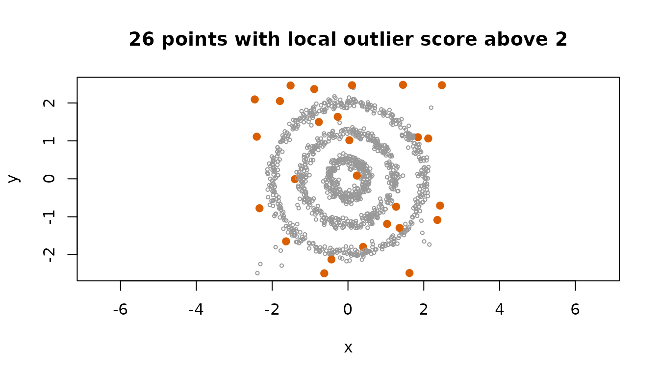

Classifying new rows

Given labelled rows, the label of a new row is a vote among its nearest labelled neighbours. query searches new rows against the reference set without them being candidates for one another.

set.seed(1)
train <- sample(nrow(x), 100)
test <- setdiff(seq_len(nrow(x)), train)

q <- shoal_knn(x[train, ], k = 5L, query = x[test, ])
votes <- matrix(as.character(species[train])[q$id], ncol = ncol(q$id))
predicted <- apply(votes, 1, function(v) names(which.max(table(v))))
table(predicted, truth = species[test])
#>             truth
#> predicted    setosa versicolor virginica
#>   setosa         16          0         0
#>   versicolor      0         19         1
#>   virginica       0          0        14

For Mahalanobis, the query rows are whitened with the reference set’s covariance, so the geometry is the reference set’s and not the query’s.

Practical notes

Both functions accept a data frame and use its numeric columns.
shoal_knn() needs k below the number of rows without a query, since a row is not its own neighbour, and at most the number of rows with one.
The tree path holds one extra copy of the data, reordered so that each leaf is contiguous in memory. On a machine where that copy matters, use search = "brute".
Both run on the package thread pool; see shoal_threads().