k-Nearest Neighbours

Finds the k nearest neighbours of every row of x among the other rows, or of every row of query among the rows of x, by an exact search in Rust. Every metric of shoal_dist() is available and the distances agree with it exactly, but only the k nearest are kept, so the memory is proportional to k times the number of rows rather than to the square of it. Where a distance matrix stops being possible somewhere in the tens of thousands of rows, a neighbour search does not.

Usage

shoal_knn(
  x,
  k,
  query = NULL,
  metric = c("euclidean", "maximum", "manhattan", "canberra", "binary", "minkowski",
    "cosine", "correlation", "mahalanobis"),
  p = 2,
  cov = NULL,
  search = c("auto", "kdtree", "brute")
)

# S3 method for class 'shoal_knn'
print(x, ...)

# S3 method for class 'shoal_knn'
plot(x, which = x$k, ...)

Arguments

x

A numeric matrix or data frame of the points to search among. Data frames are coerced to a matrix using their numeric columns (non-numeric columns are dropped). Rows containing missing or non-finite values are an error.

k

Number of neighbours to find. Must be less than nrow(x) when query is NULL, and at most nrow(x) otherwise.

query

Optional numeric matrix or data frame of points to find neighbours for, with the same columns as x. NULL (default) searches the rows of x against one another.

metric

Distance metric. One of "euclidean", "maximum", "manhattan", "canberra", "binary", "minkowski", "cosine", "correlation" or "mahalanobis".

p

Power for metric = "minkowski". Ignored otherwise. Default 2.

cov

Covariance matrix for metric = "mahalanobis", ncol(x) square and positive definite. NULL (default) uses stats::cov() of x, the reference set, whichever of x and query is being measured. Ignored for other metrics.

search

Search algorithm: "auto" (default), "kdtree" or "brute". See Details. "kdtree" is an error for a metric the tree cannot bound.

...

For plot(), further arguments to plot.default(); main, xlab and ylab given here replace the defaults. Ignored by print().

which

Which neighbour's distance to plot, between 1 and x$k. Default x$k.

Value

An object of class "shoal_knn": a list with components id, an integer matrix of row indices into x, and dist, a numeric matrix of the corresponding distances. Both have one row per point searched for and k columns, nearest first, with the row names of x or query and column names 1 to k. k, metric and search record the call, search being the algorithm actually used.

Details

Two exact searches are available and give identical results, tie order included. "brute" compares every query row with every data row, in parallel over queries; it serves every metric. "kdtree" builds an axis-aligned kd-tree and skips regions that cannot hold a nearer point; it serves every metric but "canberra" and "binary", whose distances no rectangle can bound. "cosine" and "correlation" are searched through a unit-normalised (and, for correlation, centred) copy of the rows, on which Euclidean distance orders points exactly as the metric does; the distances reported are still the metric itself. A tree prunes well in a few dimensions and hardly at all beyond about ten, where the scan is several times faster than the kd-tree searches in the dbscan and FNN packages even on one thread. The default "auto" takes the tree when the metric allows it and ncol(x) is at most 8, and the scan otherwise. The tree is built in parallel, so on a large low-dimensional set the build is a small part of the total. The tree path holds one extra copy of x, its rows reordered so that each leaf is contiguous in memory.

The conventions follow dbscan::kNN(), so code written for its results works on these. Without query, each row is excluded from its own neighbours. With query, every row of x is a candidate, so a query identical to a data row finds that row at distance zero. Neighbours are sorted by distance, and equal distances by row index, so the result is fully determined by the input. Rows with missing or non-finite values are an error rather than being dropped as shoal_dist() does: dropping rows would renumber the indices so they no longer point into the caller's matrix.

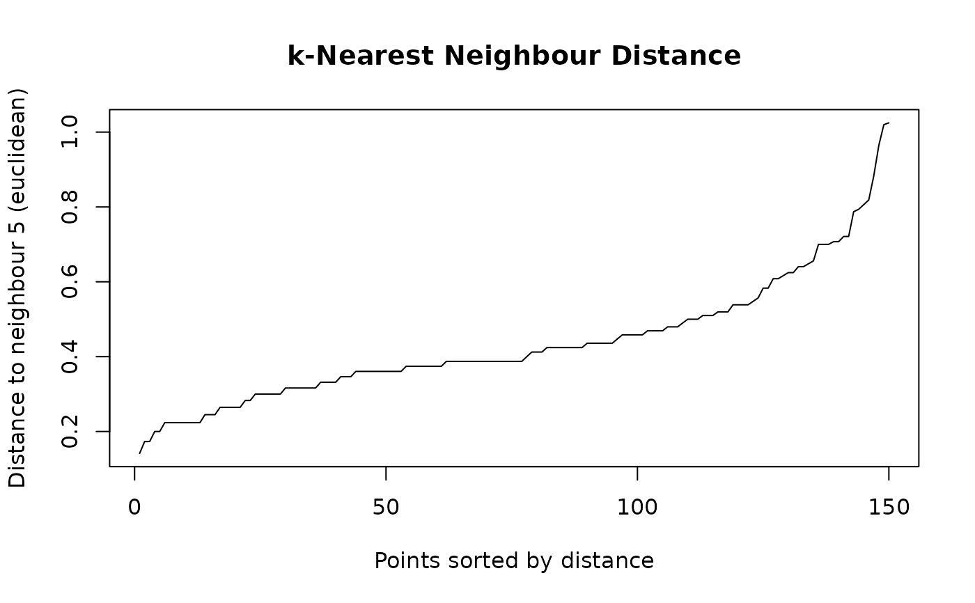
The plot() method draws each point's distance to its k-th neighbour in increasing order. The knee of that curve is the usual choice of eps for shoal_dbscan() with min_samples = k + 1; the point itself counts towards min_samples, hence the one.

See also

shoal_dist() for the full distance matrix, and shoal_dbscan(), whose eps the plot() method helps to choose.

Examples

x <- as.matrix(iris[, 1:4])
nn <- shoal_knn(x, k = 5L)
nn
#> 
#> ── k-Nearest Neighbours 
#> Metric: "euclidean", Search: "kdtree"
#> Points: 150, Neighbours: 5
#> Distance to neighbour 5: min 0.1414, median 0.3873, max 1.025
head(nn$id)
#>       1  2  3  4  5
#> [1,] 18  5 40 28 29
#> [2,] 35 46 13 10 26
#> [3,] 48  4  7 13 46
#> [4,] 48 30 31  3 13
#> [5,] 38  1 18 41  8
#> [6,] 19 11 49 45 20

# The distance to the fifth neighbour, sorted: read eps off the knee.
plot(nn)


# Neighbours of new points among the rows of x, by cosine distance.
shoal_knn(x, k = 3L, query = x[c(1, 51, 101), ], metric = "cosine")
#> 
#> ── k-Nearest Neighbours 
#> Metric: "cosine", Search: "kdtree"
#> Points: 3, Neighbours: 3
#> Distance to neighbour 3: min 1.265e-05, median 2.874e-05, max 0.0006906