Selecting cells around a point
Pick an origin cell and use a5_spherical_cap() to grab
every cell whose centre falls within a given great-circle radius. Like
a5_grid_disk(), it returns an a5_covering: a
compacted set that records its resolution. Pass it through
a5_uncompact() for the cells.
origin <- a5_lonlat_to_cell(35, 55, resolution = 14)

a5_spherical_cap(origin, radius = 5000)
#> <a5_covering[1]>
#> [1] res 14: 621 cells (105 stored)

disk <- a5_uncompact(a5_grid_disk(origin, k = 20, vertex = FALSE))
disk_vertex <- a5_uncompact(a5_grid_disk(origin, k = 20, vertex = TRUE))
cap <- a5_uncompact(a5_spherical_cap(origin, radius = 5000))
a5_grid_disk() selects cells by hop count rather than
metric distance. With vertex = FALSE (default) only
edge-sharing neighbours are traversed (4-connected), producing a diamond
shape. Setting vertex = TRUE includes corner-sharing
neighbours too (8-connected), giving a squarer footprint.
Distance heatmap
Compute the distance from the origin to every cell in the cap (or disk) and visualise it as a colour gradient.
dcap <- a5_cell_distance(origin, cap, units = "km")
ddisk <- a5_cell_distance(origin, disk, units = "km")
ddisk_vertex <- a5_cell_distance(origin, disk_vertex, units = "km")

pal <- hcl.colors(256, "Inferno")

for (info in list(
  list(s = disk, d = ddisk, lab = "Grid disk (edges)"),
  list(s = disk_vertex, d = ddisk_vertex, lab = "Grid disk (vertices)"),
  list(s = cap, d = dcap, lab = "Spherical cap")
)) {
  brk <- seq(0, max(as.numeric(info$d)), length.out = 257)
  cols <- pal[findInterval(as.numeric(info$d), brk, all.inside = TRUE)]

  plot(a5_cell_to_boundary(info$s), col = cols, border = NA, asp = 1,
       main = info$lab)
  plot(a5_cell_to_boundary(origin), border = "#ffffffff", add = TRUE)
}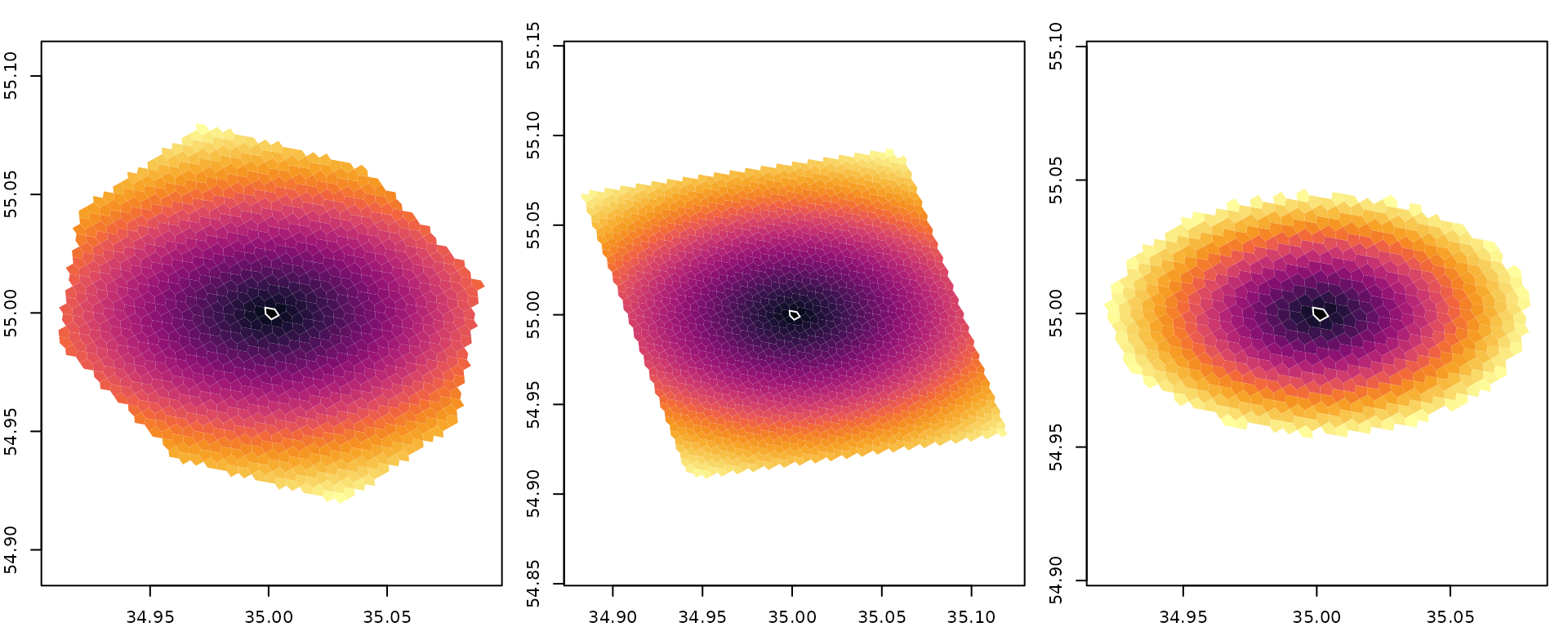
Distance radiates smoothly from the centre. Cells near the origin are dark, cells at the rim are bright. The origin cell is shown with a white border for reference.
Distance methods
a5R supports three distance methods: haversine (great-circle), geodesic (WGS84 ellipsoid via Karney 2013), and rhumb (loxodrome / constant-bearing). For short distances they are nearly identical; differences grow with distance.
wide_origin <- a5_lonlat_to_cell(35, 55, resolution = 8)
wide_cap <- a5_uncompact(a5_spherical_cap(wide_origin, radius = 500000))

hav <- a5_cell_distance(wide_origin, wide_cap, units = "m", method = "haversine")
geo <- a5_cell_distance(wide_origin, wide_cap, units = "m", method = "geodesic")

diff_m <- as.numeric(geo - hav)
brk <- seq(min(diff_m), max(diff_m), length.out = 257)
cols <- pal[findInterval(diff_m, brk, all.inside = TRUE)]

layout(matrix(c(1, 2), nrow = 1), widths = c(4, 1))
par(mar = c(2, 2, 2, 1))
plot(a5_cell_to_boundary(wide_cap), col = cols, border = NA, asp = 1,
     main = "Geodesic \u2212 Haversine (m)")

par(mar = c(9, 0, 9, 9))
image(1, seq(min(diff_m), max(diff_m), length.out = 256),
      t(seq_along(pal)), col = pal, axes = FALSE, xlab = "", ylab = "")
axis(4, las = 1)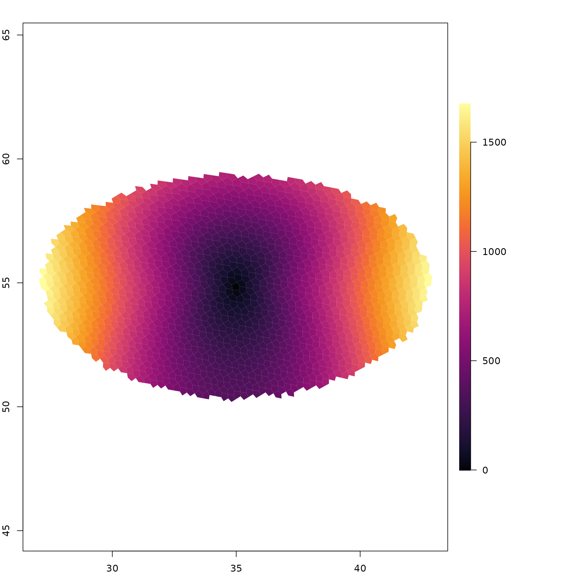
The difference is near zero at the centre and grows to ~1675 m at the rim (~500 km away).