
Index a point
Map a longitude/latitude coordinate to a cell at a given resolution (0–30). Higher resolutions produce smaller cells.
cell <- a5_lonlat_to_cell(-3.19, 55.95, resolution = 10)
cell
#> <a5_cell[1]>
#> [1] 63bb948000000000
Convert back to the cell centre point:
a5_cell_to_lonlat(cell)
#> <wk_xy[1] with CRS=OGC:CRS84>
#> [1] (-3.183746 55.9806)
Cell boundaries
Get the boundary polygon for one or more cells:
boundary <- a5_cell_to_boundary(cell)
boundary
#> <wk_wkb[1] with CRS=OGC:CRS84>
#> [1] <POLYGON ((-3.175718 55.93546, -3.145905 55.97569, -3.151641 56.01921, -3.219413 56.00818, -3.226037 55.96443, -3.175718 55.93546...>

plot(boundary, col = "#206ead20", border = "#206ead", asp = 1)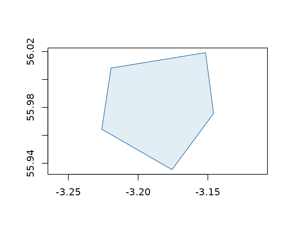
Boundaries are returned as wk_wkb vectors by default
(set format = "wkt" for WKT). Both integrate directly with
sf, terra, and other spatial tooling via the wk package.
Hierarchy and compaction
A5 is a hierarchical grid: every cell has a parent at a coarser resolution and 4 children at the next finer resolution.
parent <- a5_cell_to_parent(cell)
parent
#> <a5_cell[1]>
#> [1] 63bb960000000000

children <- a5_cell_to_children(cell)
children
#> <a5_cell[4]>
#> [1] 63bb942000000000 63bb946000000000 63bb94a000000000 63bb94e000000000
We can visualise the relationship: the parent (dark outline) contains our cell (blue fill), which in turn contains its 4 children (orange):
plot(NULL, xlim = c(-3.23, -3),  ylim = c(55.98, 55.99),
       xlab = "", ylab = "", asp = 1
       )
plot(a5_cell_to_boundary(a5_cell_to_children(cell)),
     col = "#ad6e2020", border = "#ad6e20", add = TRUE)
plot(a5_cell_to_boundary(cell), col = "#206ead40", border = "#206ead",
     lwd = 2, add = TRUE)
plot(a5_cell_to_boundary(parent), border = "#333333", lwd = 2, add = TRUE)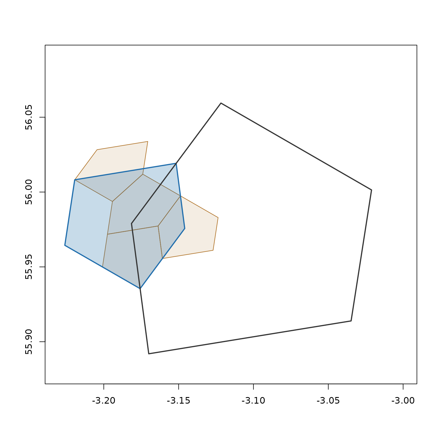
Cell area decreases geometrically: each level is roughly 4x smaller,
so the average edge length roughly halves per level.
a5_cell_edge_length_avg() gives a quick sense of cell size
when choosing a resolution.
a5_cell_area(0:5)
#> Units: [m^2]
#> [1] 4.250547e+13 8.501094e+12 2.125273e+12 5.313184e+11 1.328296e+11
#> [6] 3.320740e+10
a5_cell_edge_length_avg(0:5, units = "km")
#> Units: [km]
#> [1] 4649.1423 2343.3188 1190.1738  597.5652  299.1471  149.6100
Compact and uncompact
a5_compact() stores a set of cells as an
a5_covering: every complete group of siblings is replaced
by its parent, and the covering records the resolution it stands for, so
a5_uncompact() needs no resolution to expand it again.
children
#> <a5_cell[4]>
#> [1] 63bb942000000000 63bb946000000000 63bb94a000000000 63bb94e000000000
covering <- a5_compact(children)
covering
#> <a5_covering[1]>
#> [1] res 11: 4 cells (1 stored)

# round-trips back to the original cells
a5_uncompact(covering)
#> <a5_cell[4]>
#> [1] 63bb942000000000 63bb946000000000 63bb94a000000000 63bb94e000000000
The polygon, disk and cap functions below also return coverings. Use
a5_uncompact() when you need the cells themselves.
Traversal
Find neighbouring cells by hop count with
a5_grid_disk(), or by great-circle distance with
a5_spherical_cap(). Both return one covering per centre
cell:
disk <- a5_grid_disk(cell, k = 10)
cap <- a5_spherical_cap(cell, radius = 50000)
c(disk, cap)
#> <a5_covering[2]>
#> [1] res 10: 294 cells (69 stored) res 10: 239 cells (62 stored)

plot(a5_cell_to_boundary(a5_uncompact(cap)), col = "#6ead2020", border = "#6ead20", asp = 1)
plot(a5_cell_to_boundary(a5_uncompact(disk)), col = "#206ead20", border = "#206ead",
     asp = 1, add = TRUE)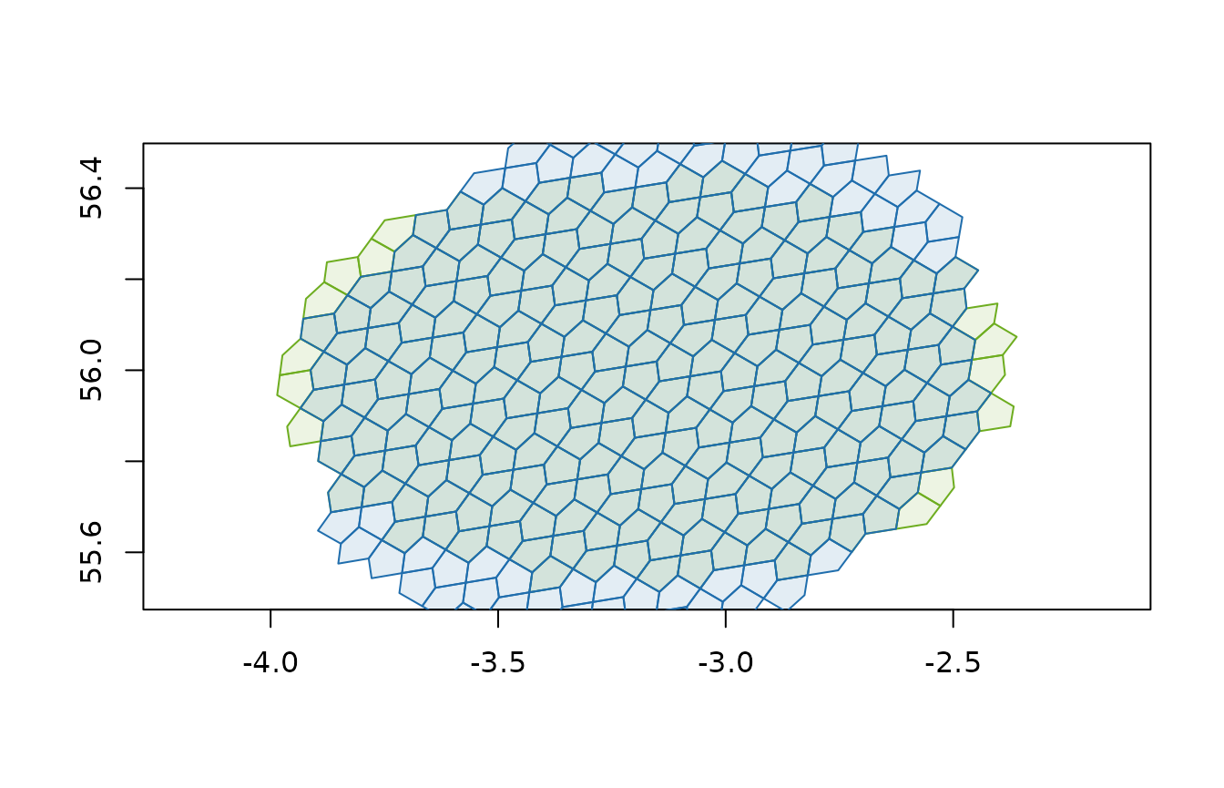
Converting geometries to a5 cells
a5_polygon_to_cells() returns the cells whose centres
lie inside a polygon. It accepts any geometry that wk can handle (a
wk::rct() bounding box, a WKT or WKB polygon, an
sf / sfc feature) and also terra
SpatVector polygons.
covering <- a5_polygon_to_cells(wk::rct(-3.3, 55.9, -3.1, 56.0), resolution = 12)
covering
#> <a5_covering[1]>
#> [1] res 12: 69 cells (36 stored)

cells <- a5_uncompact(covering)
plot(a5_cell_to_boundary(cells), col = "#206ead20", border = "#206ead", asp = 1)
A covering stores far fewer cells than it stands for: whenever four
sibling cells all sit inside the polygon, they are stored as their
parent. Stored cells are index parents, whose outlines do not nest (see
vignette("spatial-hierarchy")), so always uncompact before
drawing.
By default only cells whose centre lies inside the polygon are
returned, so cells straddling the boundary are dropped and the union of
the cells does not fully cover the polygon. Pass
containment = "overlapping" to also keep every cell that
touches the boundary, giving gap-free coverage. The overlapping set is
always a superset of the centre set.
overlapping <- a5_polygon_to_cells(wk::rct(-3.3, 55.9, -3.1, 56.0),
                                   resolution = 12, containment = "overlapping")
overlapping
#> <a5_covering[1]>
#> [1] res 12: 90 cells (36 stored)

plot(a5_cell_to_boundary(a5_uncompact(overlapping)),
     col = "#ad6e2020", border = "#ad6e20", asp = 1)
plot(a5_cell_to_boundary(cells),
     col = "#206ead40", border = "#206ead", add = TRUE)
plot(wk::rct(-3.3, 55.9, -3.1, 56.0), border = "#333333", lwd = 2, add = TRUE)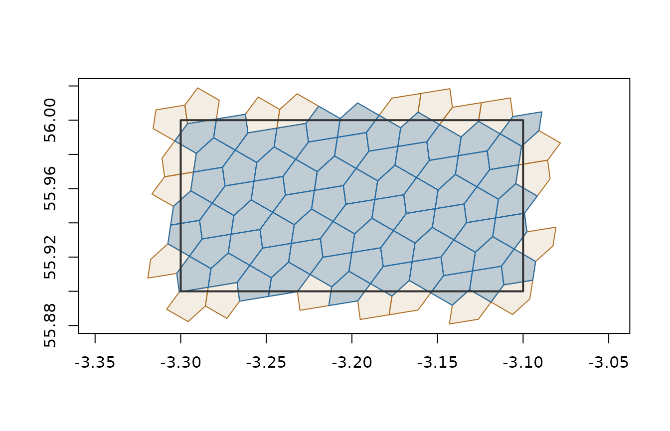
Each feature gets its own covering, so the result can be added to an
sf data frame as a column. A MULTIPOLYGON
feature’s covering holds the cells of all its parts, and a
POLYGON with holes leaves the hole cells out.
library(sf)
#> Linking to GEOS 3.12.1, GDAL 3.8.4, PROJ 9.4.0; sf_use_s2() is TRUE
demo(nc, ask = FALSE, echo = FALSE)
nc$cells <- a5_polygon_to_cells(nc, resolution = 9)
nc[1:3, c("NAME", "cells")]
#> Simple feature collection with 3 features and 2 fields
#> Attribute-geometry relationships: identity (1), NAs (1)
#> Geometry type: MULTIPOLYGON
#> Dimension:     XY
#> Bounding box:  xmin: -81.74107 ymin: 36.23388 xmax: -80.43531 ymax: 36.58965
#> Geodetic CRS:  NAD27
#>        NAME                       cells                           geom
#> 1      Ashe res 9: 11 cells (11 stored) MULTIPOLYGON (((-81.47276 3...
#> 2 Alleghany   res 9: 6 cells (6 stored) MULTIPOLYGON (((-81.23989 3...
#> 3     Surry res 9: 12 cells (12 stored) MULTIPOLYGON (((-80.45634 3...

plot(a5_cell_to_boundary(a5_uncompact(nc$cells)),
     col = "#03030320", border = "#6d20adff", asp = 1)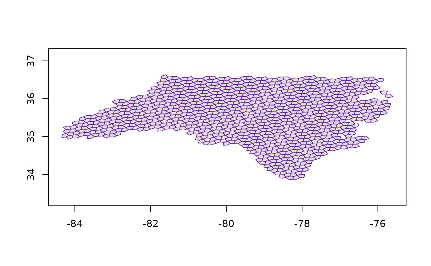
Tracing a line
a5_linestring_to_cells() returns the cells whose
pentagons are crossed by a great-circle polyline. Output is in discovery
order along the path. Consecutive waypoints are connected by
great-circle arcs, so antimeridian-crossing routes work
transparently.
Each feature gives one path: a MULTILINESTRING’s parts
are traced in order into one path, each cell kept once. For several
features, simplify = FALSE returns one path per feature as
an a5_cell_list; the default concatenates them.
To show what cell-by-cell tracing looks like, we can write a short
phrase as a MULTILINESTRING (one stroke per letter) and ask
A5 to fill in the cells:
a5R_strokes <- wk::wkt(
  "MULTILINESTRING (
    (1.8 52.5, 1.2 52.8, 0.6 52.5, 0.4 52, 0.6 51.5, 1.2 51.2, 1.8 51.5, 2 52, 1.8 52.5, 2 51.2),
    (5 53, 3.5 53, 3.5 52.2, 4 52.2, 4.7 52, 5 51.6, 4.7 51.2, 4 51, 3.5 51.1),
    (6.5 51, 6.5 53, 7.5 53, 8 52.8, 8.2 52.5, 8 52.2, 7.5 52, 6.5 52, 8.2 51)
  )"
)

cells <- a5_linestring_to_cells(a5R_strokes, resolution = 9)
length(cells)
#> [1] 182

plot(a5_cell_to_boundary(cells),
     col = "#206ead80", border = "#37af6d", asp = 1)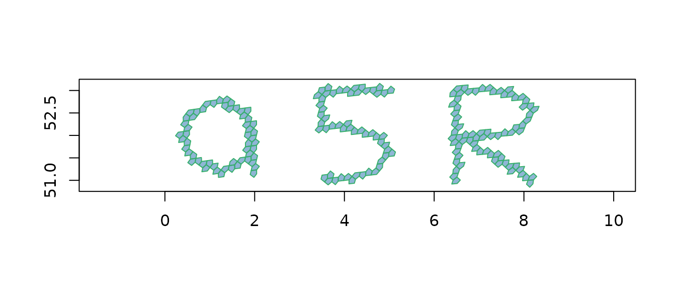
Each stroke is one part of the MULTILINESTRING; the
function walks each great-circle path in turn and joins the strokes into
one path, each cell kept once.