Moving between resolutions by location • a5R

library(a5R)
#> a5R 0.9.9.9004 • a5 crate 1.0.0-beta.3 • A5 index 1.0 • 1 thread

The index hierarchy is not spatially nested

a5_cell_to_parent() and a5_cell_to_children() follow the A5 index. A cell’s index children do not tile it: some of them lie mostly in its neighbours, and some cells inside it belong to a neighbour’s index.

a5_cell_to_supercell() and a5_cell_to_subcell() follow location instead. A fine cell belongs to the coarse cell containing its centre: that coarse cell is its supercell, and the fine cells a coarse cell holds are its subcells.

cell <- a5_lonlat_to_cell(-53.5, -19, resolution = 8)
index_kids <- a5_cell_to_children(cell, resolution = 11)
spatial_kids <- a5_uncompact(a5_cell_to_subcell(cell, resolution = 11))

outline <- a5_cell_to_boundary(cell)
lim <- wk::wk_bbox(a5_cell_to_boundary(c(index_kids, spatial_kids)))
lim <- unclass(lim)

for (panel in list(list(index_kids, "Index children"),
                   list(spatial_kids, "Subcells"))) {
  plot(NULL, xlim = c(lim$xmin, lim$xmax), ylim = c(lim$ymin, lim$ymax),
       asp = 1, axes = FALSE, xlab = "", ylab = "", main = panel[[2]])
  plot(a5_cell_to_boundary(panel[[1]]), col = "#206ead40",
       border = "#206ead", add = TRUE)
  plot(outline, border = "#333333", lwd = 2, add = TRUE)
}

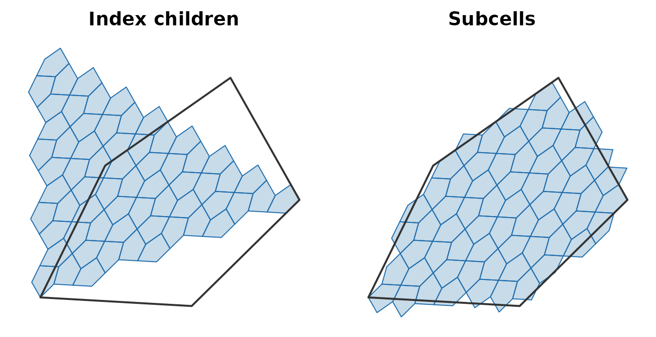
The cell has 64 index children and 66 subcells here, and only the subcells sit inside the outline. The mismatch is not rare:

set.seed(1)
fine <- a5_lonlat_to_cell(
  stats::runif(1e4, -54, -53), stats::runif(1e4, -19.5, -18.5),
  resolution = 18
)
mean(a5_cell_to_parent(fine, 15) != a5_cell_to_supercell(fine, 15))
#> [1] 0.3677

For about a third of res-18 cells, the index parent at res 15 is a neighbour of the cell they lie in, their supercell.

The upward direction shows the same thing from the other side. Here is one res-10 cell whose index parent at res 8 is not the cell it lies in:

kids <- a5_uncompact(a5_grid_disk(cell, 1), resolution = 10)
moved <- kids[a5_cell_to_parent(kids, 8) != a5_cell_to_supercell(kids, 8)]
# the clearest case: the fine cell furthest from its index parent's centre
fine_cell <- moved[which.max(a5_cell_distance(moved, a5_cell_to_parent(moved, 8)))]
index_parent <- a5_cell_to_parent(fine_cell, 8)
supercell <- a5_cell_to_supercell(fine_cell, 8)

lim <- unclass(wk::wk_bbox(a5_cell_to_boundary(c(index_parent, supercell))))

plot(NULL, xlim = c(lim$xmin, lim$xmax), ylim = c(lim$ymin, lim$ymax),
     asp = 1, axes = FALSE, xlab = "", ylab = "")
plot(a5_cell_to_boundary(index_parent), col = "#d9534f20", border = "#d9534f",
     lwd = 2, lty = 2, add = TRUE)
plot(a5_cell_to_boundary(supercell), col = "#206ead20", border = "#206ead",
     lwd = 2, add = TRUE)
plot(a5_cell_to_boundary(fine_cell), col = "#333333", border = NA, add = TRUE)
plot(a5_cell_to_lonlat(fine_cell), pch = 19, cex = 0.8, col = "white", add = TRUE)
legend("bottomright", bty = "n", lwd = 2, lty = c(2, 1),
       col = c("#d9534f", "#206ead"), legend = c("Index parent", "Supercell"))

The fine cell (dark, with its centre in white) sits inside its supercell, while its index parent is the neighbouring cell.

Aggregating to a coarser grid

Take a complete res-18 layer over a small area containing a circular patch, such as a stand of forest: cells inside the patch have value 1, cells outside have value 0. Average it to res 15 under each rule.

area <- a5_lonlat_to_cell(-53.5, -19, resolution = 12)
layer <- a5_uncompact(a5_grid_disk(area, 1), resolution = 18)
length(layer)
#> [1] 24576

centre <- unclass(a5_cell_to_lonlat(area))
in_patch <- function(p) {
  p <- unclass(p)
  as.numeric((p$x - centre$x)^2 + (p$y - centre$y)^2 < 0.004^2)
}
fine <- data.frame(value = in_patch(a5_cell_to_lonlat(layer)))

mean_by <- function(cell, value) {
  stats::aggregate(list(value = value), list(cell = format(cell)), mean)
}
by_index <- mean_by(a5_cell_to_parent(layer, 15), fine$value)
by_super <- mean_by(a5_cell_to_supercell(layer, 15), fine$value)

For a reference that uses neither hierarchy, drop two million random points on the area, place each directly in its res-15 cell, and take the share of points per cell that fall in the patch. This estimates each coarse cell’s true patch fraction.

set.seed(1)
bb <- unclass(wk::wk_bbox(a5_cell_to_lonlat(layer)))
pts <- list(x = stats::runif(2e6, bb$xmin, bb$xmax),
            y = stats::runif(2e6, bb$ymin, bb$ymax))
truth <- mean_by(a5_lonlat_to_cell(pts$x, pts$y, resolution = 15), in_patch(pts))
names(truth)[2] <- "truth"

error <- function(agg) {
  m <- merge(agg, truth)
  m <- m[m$value > 0 | m$truth > 0, ]
  round(c(mean = mean(abs(m$value - m$truth)), max = max(abs(m$value - m$truth))), 3)
}
error(by_index)
#>  mean   max 
#> 0.086 0.338
error(by_super)
#>  mean   max 
#> 0.008 0.057

Aggregating by index parent misstates the patch fraction of the cells it touches by about a tenth on average, and by a third at worst, because each coarse cell averages fine cells from its neighbours. Aggregating by supercell is off only by the sampling noise of the reference. format() supplies a grouping key here because base grouping functions cannot group an a5_cell vector directly (see vignette("internal-cell-representation")).

Mapping the reference fractions, and each rule’s error against them, shows where the index rule goes wrong:

grid <- merge(merge(truth, by_index, all.x = TRUE), by_super,
              by = "cell", all.x = TRUE, suffixes = c("_index", "_super"))
grid[is.na(grid)] <- 0
cells <- a5_cell(grid$cell)
xy <- unclass(a5_cell_to_lonlat(cells))
near <- (xy$x - centre$x)^2 + (xy$y - centre$y)^2 < 0.006^2
grid <- grid[near, ]
boundaries <- a5_cell_to_boundary(cells[near])
lim <- unclass(wk::wk_bbox(boundaries))

fraction_pal <- hcl.colors(101, "Greens", rev = TRUE)
error_pal <- hcl.colors(101, "Blue-Red 3")
ring <- seq(0, 2 * pi, length.out = 200)
error_col <- function(e) error_pal[round(pmin(pmax(e / 0.4, -1), 1) * 50) + 51]

for (panel in list(
  list(fraction_pal[round(grid$truth * 100) + 1], "Reference fraction"),
  list(error_col(grid$value_index - grid$truth), "Index parent error"),
  list(error_col(grid$value_super - grid$truth), "Supercell error")
)) {
  plot(NULL, xlim = c(lim$xmin, lim$xmax), ylim = c(lim$ymin, lim$ymax),
       asp = 1, axes = FALSE, xlab = "", ylab = "", main = panel[[2]])
  plot(boundaries, col = panel[[1]], border = "white", lwd = 0.5, add = TRUE)
  lines(centre$x + 0.004 * cos(ring), centre$y + 0.004 * sin(ring),
        col = "#333333", lwd = 1.5)
}

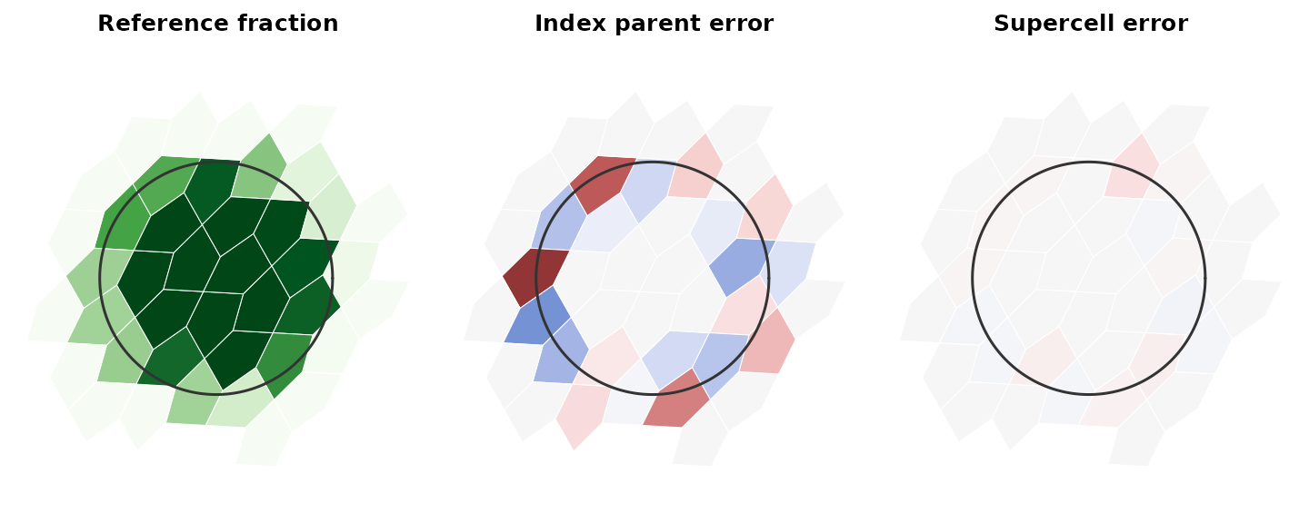
The left panel shades each res-15 cell by its patch fraction, from white (none) to dark green (all), with the patch outline in dark grey. The other two show aggregated minus reference, from blue (0.4 or more too low) through grey to red (0.4 or more too high). Index aggregation is wrong in both directions all along the patch edge, where a coarse cell’s index children fall on the other side of the edge from the cell itself. Supercell aggregation is grey apart from faint tints, which are sampling noise in the reference.

Expanding coarse cells

The downward direction is the exact inverse. a5_cell_to_subcell() returns one covering per coarse cell: a compacted set that records its resolution (see ?a5_covering). Expanding the subcells of a set of coarse cells gives each fine cell once, inside the coarse cell whose centre rule claims it:

patch <- a5_uncompact(a5_grid_disk(cell, 1))
sub <- a5_cell_to_subcell(patch, resolution = 11)
sub
#> <a5_covering[6]>
#> [1] res 11: 62 cells (29 stored) res 11: 62 cells (29 stored)
#> [3] res 11: 62 cells (29 stored) res 11: 66 cells (33 stored)
#> [5] res 11: 66 cells (33 stored) res 11: 62 cells (29 stored)

kids <- a5_uncompact(sub, simplify = FALSE)
lengths(kids)
#> [1] 62 62 62 66 66 62

all_kids <- unlist(kids)
vctrs::vec_duplicate_any(all_kids)
#> [1] FALSE
all(a5_cell_to_supercell(all_kids, 8) == rep(patch, lengths(kids)))
#> [1] TRUE

Counts vary slightly from cell to cell but average 4^3 = 64 for these three resolution steps, as for index children. Each covering stores far fewer cells than it stands for; uncompact before drawing, as the stored cells are index parents.

Which to use

Use the index functions for operations on ids: compaction, id ranges and curve ordering. Use supercells and subcells whenever values move between resolutions and must stay where they are on the ground.

Supercells and subcells cost more. The index functions are bit operations; a5_cell_to_supercell() locates each centre, in well under half the time of a5_lonlat_to_cell(). Both run in parallel with a5_set_threads().