Remote sources: storage, authentication and windows • cptkirk

library(cptkirk)

cptkirk reads Cloud-Optimised GeoTIFFs straight from cloud object stores — S3, Google Cloud Storage, Azure, plain HTTP(S), or local disk. This article covers the three things people ask first: how a source is addressed, how it authenticates, and how to pull pixels (a window, or a whole reprojected AOI) into R.

We use three public datasets, chosen to span the awkward cases:

Dataset	Access	CRS	Type
Alpha Earth Foundations embeddings	plain `https://` (no auth)	UTM 36S	Int8, 64 bands
Sentinel-2 L2A (AWS Open Data)	`s3://` (anonymous + region)	UTM	Byte / UInt16, one COG per band
GEBCO 2024 bathymetry	plain `https://` (no auth)	EPSG:4326	Int16, global

A source is a single URL

Where libraries like obstore / async-tiff separate a store (bucket, region, credentials) from a path (the object key), cptkirk takes one self-contained URL and works out the rest. The scheme (and, for AWS, the host) selects the backend; the rest is the object key.

aef <- paste0(
  "https://data.source.coop/tge-labs/aef/v1/annual/2021/36S/",
  "xekh5rjs4wg6wb9b4-0000000000-0000000000.tiff"
)
cog_info(aef)
#> ── cog_info ────────────────────────────────────────────────────────────────────
#> <https://data.source.coop/tge-labs/aef/v1/annual/2021/36S/xekh5rjs4wg6wb9b4-0000000000-0000000000.tiff>
#> size: 8192 x 8192 px (67.1 Mpx)
#> bands: 64 Int8
#> resolution: 10 (CRS units)
#> crs: EPSG:32736
#> nodata: -128
#> overviews: 13 (8192x8192, 4096x4096, 2048x2048, 1024x1024, 512x512, 256x256,
#> 128x128, 64x64, 32x32, 16x16, 8x8, 4x4, 2x2, 1x1)
#> band names: "A00", "A01", "A02", "A03", "A04", "A05", …, "A62", and "A63"

cog_info() reads only the header and IFDs — no pixels — so it is a cheap way to understand a file before fetching anything.

Authentication comes from the environment

cptkirk never takes credentials as arguments; it reads them from the environment, so secrets stay out of your scripts. It honours the same variables as GDAL’s /vsi* drivers, so a setup that already works with GDAL needs no change: AWS_ACCESS_KEY_ID / AWS_SECRET_ACCESS_KEY / AWS_REGION, AWS_NO_SIGN_REQUEST=YES for public buckets, AWS_S3_ENDPOINT for a custom endpoint, GOOGLE_APPLICATION_CREDENTIALS, AZURE_STORAGE_ACCOUNT, and so on. The object_store-native spellings (AWS_SKIP_SIGNATURE, …) work too; where the two differ, cptkirk translates the GDAL name. Only non-secret knobs are translated R-side – credentials pass straight from the environment to the reader.

Mapping from the obstore store object:

`obstore`	cptkirk
`S3Store("bucket", region = "us-west-2", skip_signature = True)`	`Sys.setenv(AWS_REGION = "us-west-2", AWS_SKIP_SIGNATURE = "true")` (or GDAL’s `AWS_NO_SIGN_REQUEST = "YES"`)
`path = "key/within/bucket"`	fold into the URL: `s3://bucket/key/within/bucket`
`GeoTIFF.open(path, store = store)`	`cog_info(url)` / `ck_read(url)` / `ck_warp(url, dst)`

Two situations:

Plain https:// on a non-AWS host (the AEF tile above, GEBCO below) uses the HTTP backend and needs nothing.
AWS-hosted data — whether you write s3://… or https://….amazonaws.com/… — routes to the S3 backend, which signs requests. For a public bucket, switch signing off and set the region:

Sys.setenv(AWS_REGION = "us-west-2", AWS_SKIP_SIGNATURE = "true")

scene <- paste0(
  "s3://sentinel-cogs/sentinel-s2-l2a-cogs/12/S/UF/2022/6/",
  "S2B_12SUF_20220609_0_L2A/"
)
cog_info(paste0(scene, "TCI.tif"))
#> ── cog_info ────────────────────────────────────────────────────────────────────
#> <s3://sentinel-cogs/sentinel-s2-l2a-cogs/12/S/UF/2022/6/S2B_12SUF_20220609_0_L2A/TCI.tif>
#> size: 10980 x 10980 px (120.6 Mpx)
#> bands: 3 Byte
#> resolution: 10 (CRS units)
#> crs: EPSG:32612
#> nodata: 0
#> overviews: 4 (10980x10980, 5490x5490, 2745x2745, 1373x1373, 687x687)
#> band names: "band_01", "band_02", and "band_03"

The selection is by host, not scheme: a *.amazonaws.com URL is treated as S3 even over https, so it still needs the no-sign flag here. Either spelling works — AWS_SKIP_SIGNATURE = "true" (object_store) or AWS_NO_SIGN_REQUEST = "YES" (GDAL); cptkirk normalises the GDAL YES/NO form for you.

Reading a window into R

ck_read() is ck_warp() that returns a base-R array instead of writing a file. With no t_srs or tr it reads the native window directly (no GDAL); the returned matrix/array carries geotransform, crs and nodata attributes, so it is self-describing.

If you think in source pixel offsets (like async-tiff’s Window(col_off, row_off, width, height)), convert them to a target extent with the geotransform and hand that to ck_read():

gt <- cog_info(paste0(scene, "B04.tif"))$geotransform

col_off <- 4096L; row_off <- 2048L; width <- 512L; height <- 512L
te <- c(gt[1] +  col_off            * gt[2],   # xmin
        gt[4] + (row_off + height)  * gt[6],   # ymin (gt[6] is negative)
        gt[1] + (col_off + width)   * gt[2],   # xmax
        gt[4] +  row_off            * gt[6])   # ymax

a <- ck_read(paste0(scene, "B04.tif"), te = te)   # native window, no reprojection
dim(a)
#> [1] 512 512
str(attributes(a))
#> List of 4
#>  $ dim         : int [1:2] 512 512
#>  $ geotransform: num [1:6] 340960 10 0 4079560 0 ...
#>  $ crs         : chr "EPSG:32612"
#>  $ nodata      : num 0

The array maps onto async-tiff’s RasterArray: the values are data, dim(a) is shape, attr(a, "geotransform") is transform, attr(a, "crs") is crs, and attr(a, "nodata") stands in for mask (derive one with a == attr(a, "nodata")).

Building a stack from per-band COGs

Sentinel-2 L2A stores one COG per band, at each band’s native resolution (10 m for the visible/NIR bands, 20 m for the SWIR bands). To assemble an analysis-ready stack you read each band onto the same grid. Because ck_read() aligns output to the tr grid by default, bands fetched with the same te/tr come back co-registered — even when their native resolutions differ, GDAL resamples each onto the common grid:

te20 <- c(gt[1] + 4096 * gt[2], gt[4] - (4096 + 512) * abs(gt[6]),
          gt[1] + (4096 + 512) * gt[2], gt[4] - 4096 * abs(gt[6]))

bands <- c(B08 = "B08.tif", B04 = "B04.tif", B11 = "B11.tif")  # 10 m, 10 m, 20 m
layers <- lapply(bands, function(b) {
  ck_read(paste0(scene, b), te = te20, tr = c(20, 20), r = "bilinear")
})
vapply(layers, dim, integer(2))         # identical dims -> co-registered
#>      B08 B04 B11
#> [1,] 256 256 256
#> [2,] 256 256 256

stack <- array(0, dim = c(dim(layers[[1]]), length(layers)))
for (k in seq_along(layers)) stack[, , k] <- layers[[k]]
dim(stack)
#> [1] 256 256   3

(cptkirk’s multi-source form, ck_warp(src = c(tile_a, tile_b), …), is a spatial mosaic of the same data across adjacent tiles — not a band stack, so combining separate band files is a “read each, bind” as above.)

Reprojecting on the way out

The same call warps as it reads. GEBCO is global and in EPSG:4326; here we pull a region of it reprojected to Web Mercator and resampled to 2 km, fetching only the overview and window that target needs:

gebco <- "https://projects.pawsey.org.au/idea-gebco-tif/GEBCO_2024.tif"

out <- ck_warp(
  gebco, tempfile(fileext = ".tif"),
  t_srs = "EPSG:3857",
  te    = c(110, -45, 155, -10),   # Australia, in EPSG:4326 ...
  te_srs = "EPSG:4326",            # ... so name the extent's CRS
  tr    = c(2000, 2000),
  r     = "average"
)
#> ! GDAL WARNING 1: Clamping output bounds to (-20037508.342789,-20037508.342789) -> (20037508.342789, 20037508.342789)
ds <- new(gdalraster::GDALRaster, out)
gdalraster::plot_raster(ds, legend = TRUE)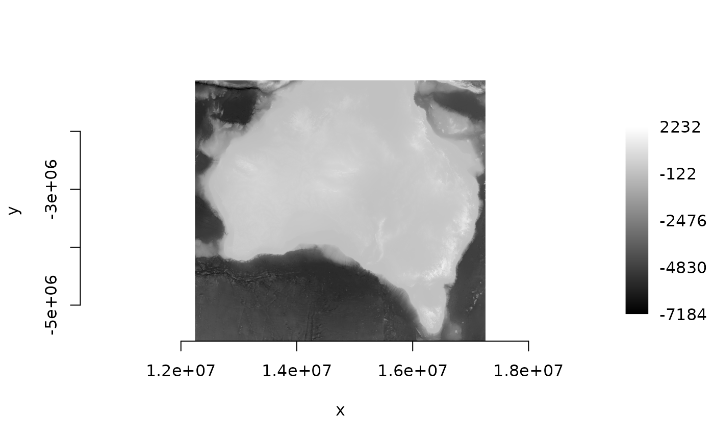

ds$close()

The remote read fetched only the tiles covering that extent, at the overview matching 2 km, then handed the reprojection and resampling to GDAL.