Get started with a5view
a5view.Rmda5view draws A5 cells, the pentagonal
cells of a global, equal-area grid. a5R makes and works with
the cells; a5view draws them in two ways: geom_a5() adds
them to a ggplot2 plot, and a5_view() puts them on an
interactive web map. Both take the same input:
- an
a5_cellvector, or a data frame with ana5_cellcolumn, one cell per row; - an
a5_coveringvector, or a data frame with ana5_coveringcolumn, one set of cells per row (see Coverings).
Cells
a5_lonlat_to_cell() gives the cell that contains a point
at a chosen resolution. Resolution 0 has 12 cells over the globe, and
each further resolution has about four times as many; at resolution 18 a
cell is about 22 m across. s2_santiago, which ships with
a5view, holds a Sentinel-2 image of central Santiago, Chile, already
indexed to resolution-18 cells:
head(s2_santiago)
#>               cell  B02  B03  B04  B08
#> 1 32b5c12040800000 1919 2165 2432 2445
#> 2 32b5c12041800000 1259 1575 1831 2254
#> 3 32b5c12042800000 2047 2414 2597 2807
#> 4 32b5c12043800000  989 1228 1441 2077
#> 5 32b5c12044800000 1305 1527 1663 2179
#> 6 32b5c12045800000 1121 1355 1569 2023
In ggplot2 the cells go to the cell aesthetic, and every
other aesthetic works as usual. Here the fill is NDVI, a vegetation
index computed from the near-infrared and red bands:
s2_santiago$NDVI <- with(s2_santiago, (B08 - B04) / (B08 + B04))

ggplot(s2_santiago, aes(cell = cell, fill = NDVI)) +
  geom_a5() +
  scale_fill_distiller(palette = "Greens", direction = 1)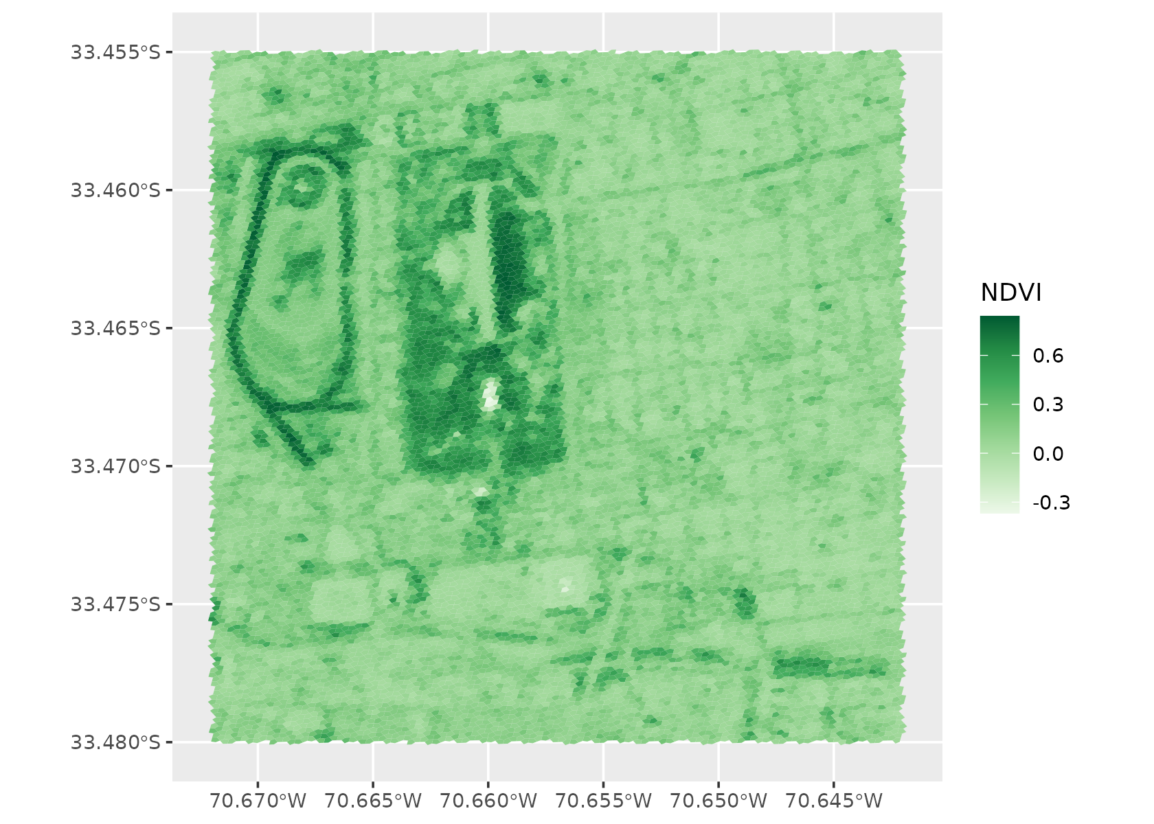
a5_view() takes the same data. fill names a
column, or an expression of columns, as aes() does:
a5_view(s2_santiago, fill = NDVI, opacity = 0.8)Hover over a cell to see its id and value; click to pin it.
Coverings
A covering is a set of cells at one resolution that stands
for an area: the cells within a radius of a point, around a cell, or
inside a polygon. a5R builds them with a5_spherical_cap(),
a5_grid_disk() and a5_polygon_to_cells().
A covering is stored compacted: wherever all four children of a parent cell are present, the parent is stored in their place, so a large covering stores far fewer cells than it stands for. a5R’s coverings article covers this in detail.
Here is the area within 900 m of the centre of Parque O’Higgins, at resolution 16 (cells about 73 m across):
centre <- a5_lonlat_to_cell(-70.657, -33.4675, resolution = 16)
park <- a5_spherical_cap(centre, radius = 900)
park
#> <a5_covering[1]>
#> [1] res 16: 324 cells (81 stored)

# cells it stands for, and cells it stores
a5_count(park)
#> [1] 324
length(a5_covering_stored(park))
#> [1] 81
Compacted or uncompacted
a5view draws what it is given. A covering is drawn as the cells it
stores, at their mixed resolutions; a5_uncompact() expands
it to the cells it stands for, all at resolution 16. Which to draw is
your choice: the compacted form shows how the covering is stored, the
uncompacted form the area it covers.
stored <- a5_covering_stored(park)
expanded <- a5_uncompact(park)
both <- data.frame(
  form = rep(c("compacted", "uncompacted"), c(length(stored), length(expanded))),
  cell = c(stored, expanded)
)
both$resolution <- factor(a5_get_resolution(both$cell))

ggplot(both, aes(cell = cell, fill = resolution)) +
  geom_a5(colour = "white", linewidth = 0.2) +
  facet_wrap(~form) +
  scale_fill_viridis_d(direction = -1)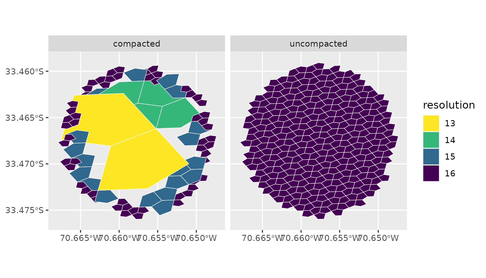
The stored parents do not line up exactly with the children they stand for: A5 cells nest in the index, not in space, so a parent’s outline overlaps its neighbours in places and leaves gaps in others. Drawn uncompacted, the covering shows exactly the cells it holds.
The covering can go straight to geom_a5() or
a5_view(), with no data frame:
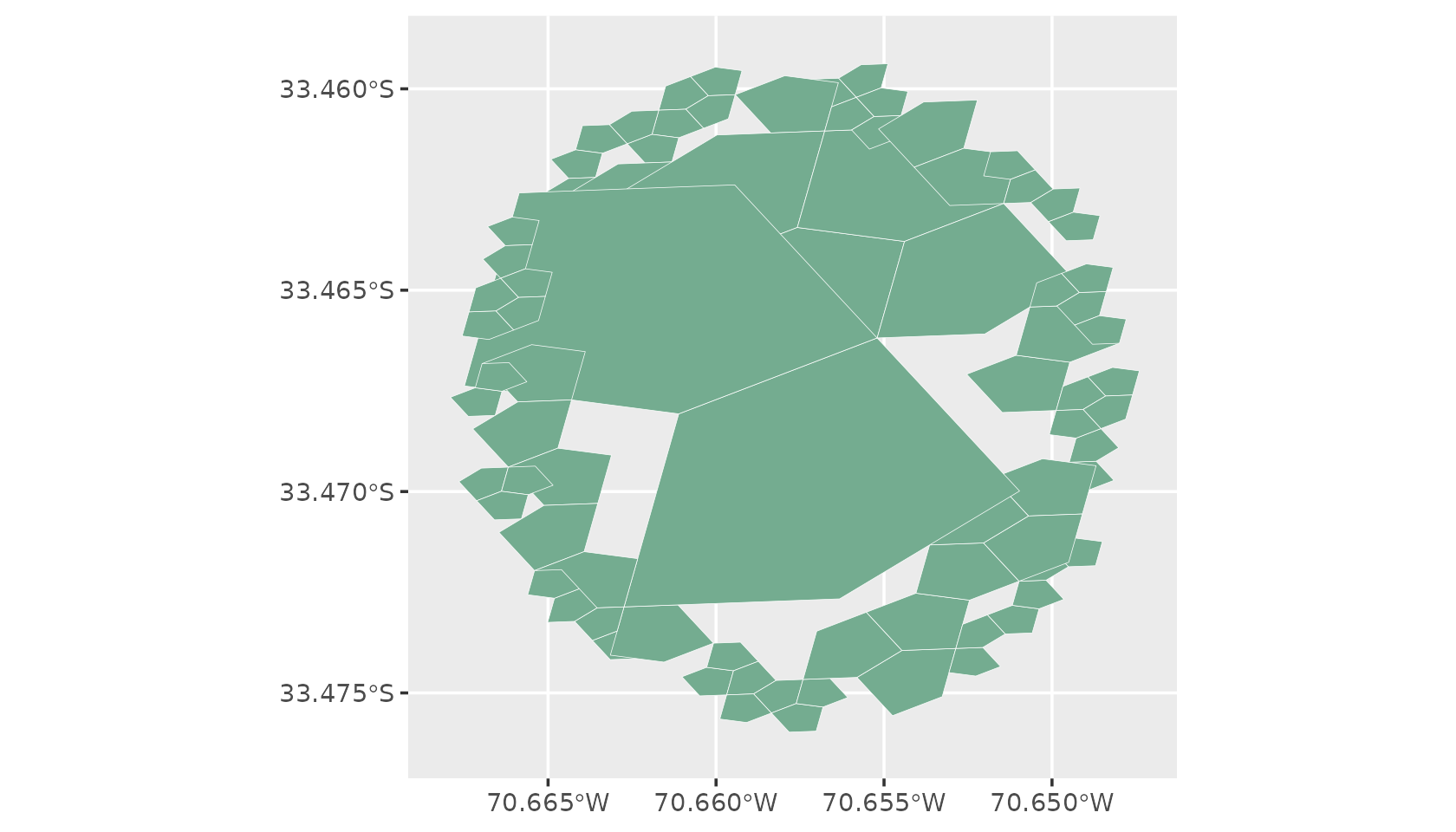
a5_view(park, border = "white")And uncompacted:
a5_view(a5_uncompact(park), border = "white")Coverings in a data frame
An a5_covering vector holds one covering per element, so
it fits in a data frame column next to the attributes of each area.
a5view repeats each row once per stored cell, so the other columns map
to aesthetics as usual. Here are three sites around the park, each with
its own radius:
sites <- data.frame(
  name = c("A", "B", "C"),
  lon = c(-70.657, -70.667, -70.649),
  lat = c(-33.4675, -33.4605, -33.4745),
  radius = c(700, 400, 250)
)
centres <- a5_lonlat_to_cell(sites$lon, sites$lat, resolution = 16)
sites$area <- do.call(c, lapply(seq_len(nrow(sites)), function(i) {
  a5_spherical_cap(centres[i], radius = sites$radius[i])
}))

ggplot(sites, aes(cell = area, fill = name)) +
  geom_a5(colour = "white", linewidth = 0.2)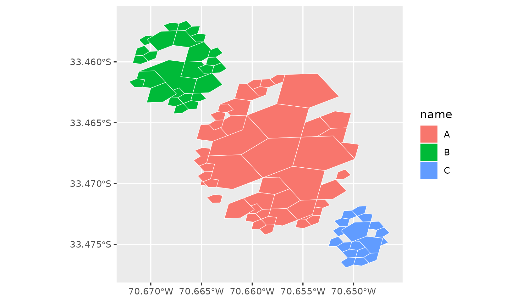
On the map, colour the sites by a numeric column, and list other
columns to show on hover with tooltip. Hovering finds cells
at every resolution present, so a compacted covering’s parents show
their row too.
a5_view(sites, fill = radius, tooltip = "name")To draw each site uncompacted, expand the coverings and repeat each
row’s attributes once per cell; a5_count() gives the number
of cells in each:
cells <- data.frame(
  name = rep(sites$name, a5_count(sites$area)),
  cell = a5_uncompact(sites$area)
)

ggplot(cells, aes(cell = cell, fill = name)) +
  geom_a5(colour = "white", linewidth = 0.2)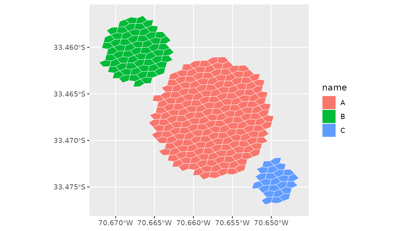
Coverings and data
A covering is also a filter. a5_contains() tests cells
against a covering without expanding it, when the cells are at the
covering’s resolution. Build the covering at the resolution of the data,
resolution 18 here, to select the image cells within 400 m of the park
centre:
centre18 <- a5_lonlat_to_cell(-70.657, -33.4675, resolution = 18)
near <- a5_spherical_cap(centre18, radius = 400)
inside <- s2_santiago[a5_contains(near, s2_santiago$cell), ]
nrow(inside)
#> [1] 1011

ggplot(inside, aes(cell = cell, fill = NDVI)) +
  geom_a5() +
  scale_fill_distiller(palette = "Greens", direction = 1)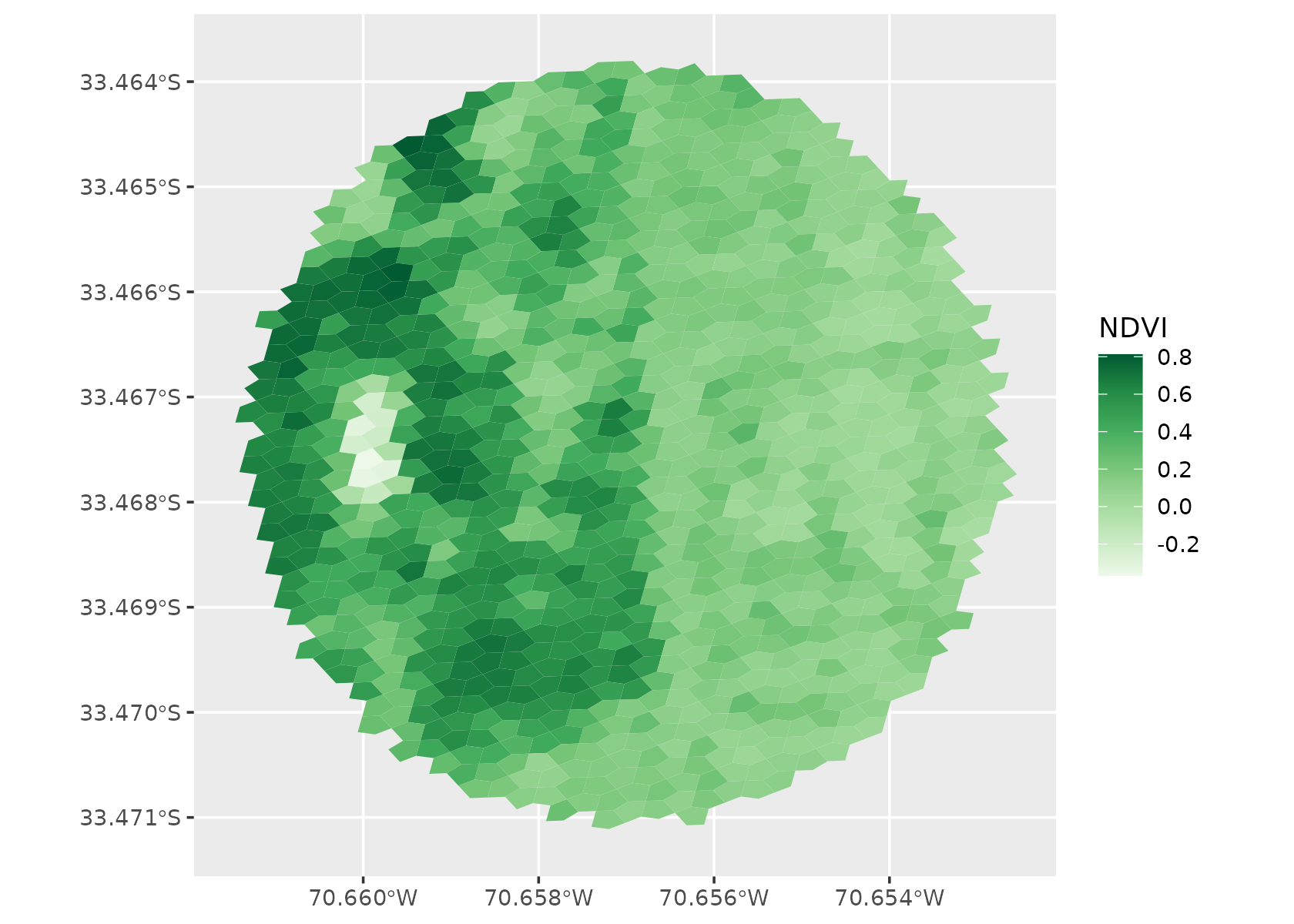
a5_uncompact() can also expand to a finer resolution
than the covering’s own, for example to match coarse coverings to fine
data: a5_uncompact(park, resolution = 18) gives the
resolution-18 cells inside the resolution-16 covering.
Large datasets
By default a5_view() sends every cell to the browser.
For large datasets, aggregate = "mean" or
"rep_child" builds a level-of-detail pyramid in which
coarser cells summarise their children, and
a5_build_pyramid() saves one to a parquet file for
a5_view_pyramid(). A pyramid is built from cells at one
resolution, so uncompact a covering before aggregating it.